---
title: "Week 10 figures - Lectures 17 and 18"
date: 2026-03-10
categories: [generalized linear model, logistic regression]
citation:
url: https://winter-2026.envs-193ds.com/lecture/lecture_week-10.html
---
```{r}
# cleaning
library(tidyverse)

# visualization
theme_set(theme_bw() +
            theme(panel.grid = element_blank(),
                  axis.text = element_text(size = 18),
                  axis.title = element_text(size = 18),
                  text = element_text(family = "Lato"),
                  strip.text = element_text(size = 16),
                  strip.background = element_rect(fill = "#FFFFFF")))
library(patchwork)
library(ggeffects)
library(flextable)
library(GGally)
library(equatiomatic)

# data
library(palmerpenguins)

# analysis
library(car)
library(performance)
library(broom)
library(DHARMa)
library(MuMIn)
library(lmtest)
library(emmeans)

bats <- read_csv(here::here("data",
                            "Cleaned Inf MYLU Band Recap Data for Ecotraps Analysis.csv"))
```
# math notation
### simple linear regression
$$
E[y_i] = a + bx_i
$$
$$
var[y_i] = s^2
$$
### generalized form:
$$
E[y_i] = a + bx_i
$$
$$
var[y_i] = v(E[y_i])
$$
## GLM structure using Gaussian example
### random component
$$
Y_i \sim N(\mu_i, \sigma^2)
$$
$$
Y_i \sim Normal(\mu_i, \sigma^2)
$$
### systematic component
$$
\eta_i = \sum^{p-1}_{n = 0}\beta_jx_{ij}
$$
$$
\mu_i = \beta_0 + \beta x_i
$$
### link
$$
\eta = g(\mu_i)
$$
## GLM structure using binary example
### random
$$
E(Y) = p
$$
### systematic
### link
$$
\eta = g(p) = log(\frac{p_i}{1 - p_i})
$$
$$
log(\frac{p_i}{1 - p_i}) = \beta_0 + \beta_1 x_i
$$
$$
Y_i \sim Binomial(p_i)
$$
$$
\eta = logit(p_i) = log(\frac{p_i}{1 - p_i})
$$
### inverse logit
$$
\frac{1}{1+e^{-x}}
$$
### model equation
$$
log(\frac{p}{1-p}) = 13.0974 - 0.6741 \times distance
$$
## bat equations
$$
log(\frac{p}{1-p}) = 5.9443 - 0.7178x
$$
$$
log(\frac{p}{1-p}) = 0.9239 - 0.2039x
$$
# binomial/bernoulli example
```{r}
set.seed(666)
lizard <- tibble(
  pushup = c(rep(1, 30), rep(0, 30)),
  distance = c(rnorm(n = 20, mean = 10, sd = 2),
               rnorm(n = 20, mean = 20, sd = 2),
               rnorm(n = 20, mean = 30, sd = 2))
) %>%
  mutate(distance = round(distance, 1))

slice_sample(lizard, n = 10)
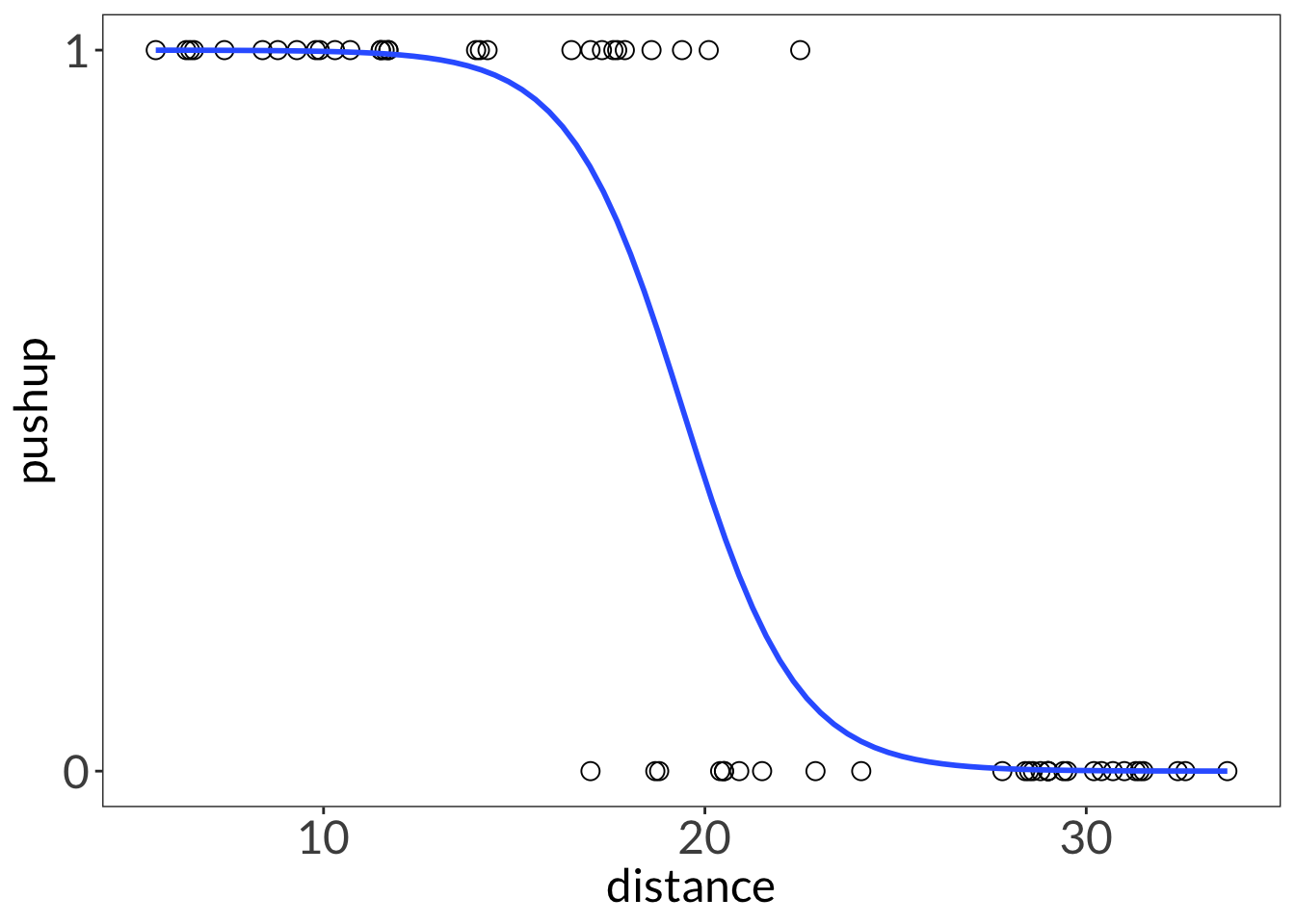
ggplot(lizard,
       aes(x = distance,
           y = pushup)) +
  geom_point(size = 3,
             shape = 21) +
  scale_y_continuous(limits = c(0, 1),
                     breaks = c(0, 1)) +
  geom_smooth(method = "glm",
              method.args = list(family = "binomial"),
              se = FALSE,
              linewidth = 1)
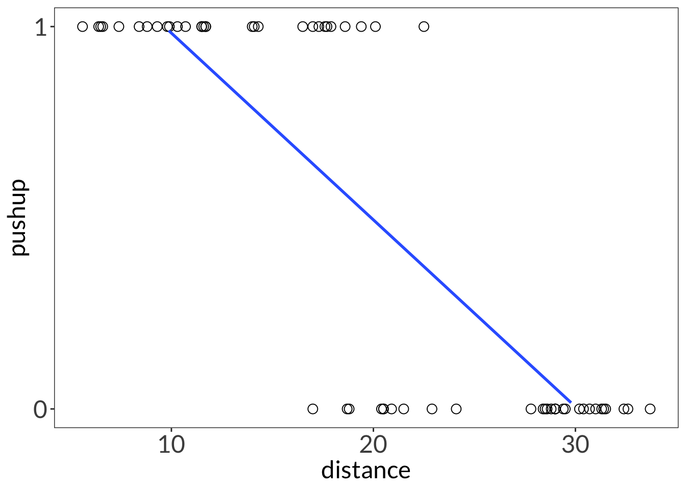
ggplot(lizard,
       aes(x = distance,
           y = pushup)) +
  geom_point(size = 3,
             shape = 21) +
  scale_y_continuous(limits = c(0, 1),
                     breaks = c(0, 1)) +
  geom_smooth(method = "lm",
              se = FALSE,
              linewidth = 1)
liz_mod <- glm(pushup ~ distance,
               data = lizard,
               family = "binomial")

summary(liz_mod)
plogis(13.0974)
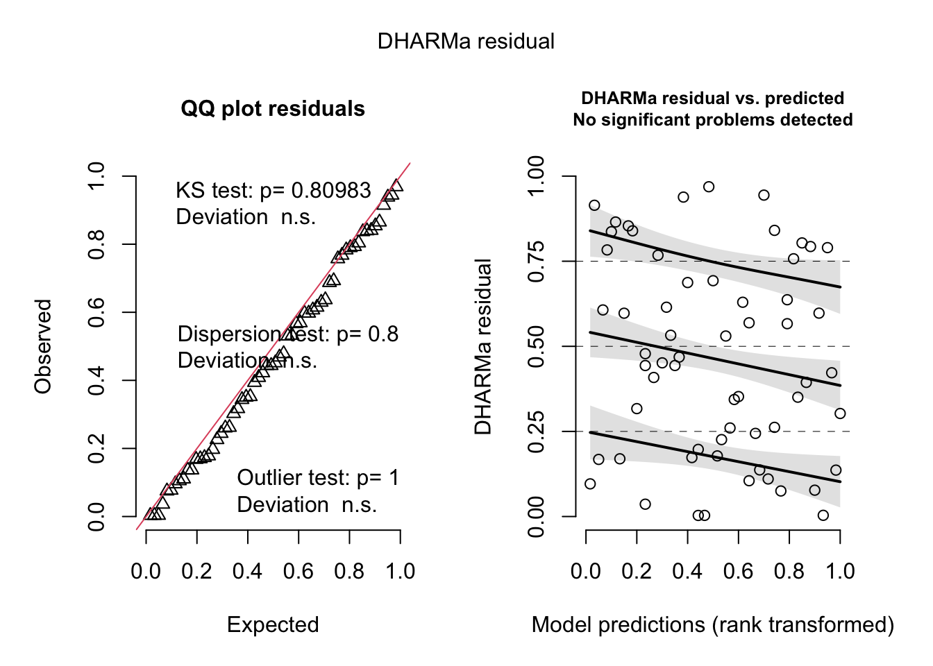
plot(
  simulateResiduals(liz_mod)
)
confint(liz_mod)
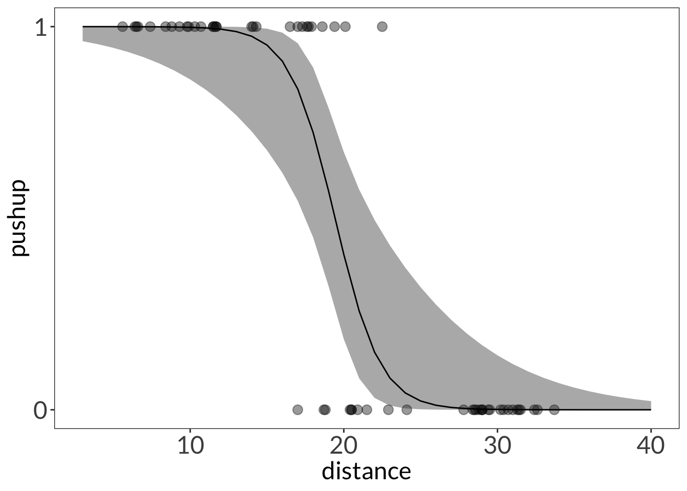
mod_preds <- ggpredict(liz_mod,
                       terms = "distance [3:40 by = 1]")

ggplot(lizard,
       aes(x = distance,
           y = pushup)) +
  geom_point(size = 3,
             alpha = 0.4) +
  geom_ribbon(data = mod_preds,
              aes(x = x,
                  y = predicted,
                  ymin = conf.low,
                  ymax = conf.high),
              alpha = 0.4) +
  geom_line(data = mod_preds,
            aes(x = x,
                y = predicted)) +
  scale_y_continuous(limits = c(0, 1),
                     breaks = c(0, 1))
# what is the probability of a pushup at 20cm?
ggpredict(liz_mod,
          terms = "distance [0]")
# what is the probability of a pushup at 20cm?
ggpredict(liz_mod,
          terms = "distance [20]")
# what is the probability of a pushup at 10cm?
ggpredict(liz_mod,
          terms = "distance [10]")
# what is the probability of a pushup at 30cm?
ggpredict(liz_mod,
          terms = "distance [30]")
# what is the probability of a pushup at 20cm?
predict(liz_mod,
        newdata = data.frame(distance = 20),
        type = "response")
r.squaredLR(liz_mod)
gtsummary::tbl_regression(liz_mod)
gtsummary::tbl_regression(liz_mod,
                          exponentiate = TRUE)
as_flextable(liz_mod)
```
# negative binomial example
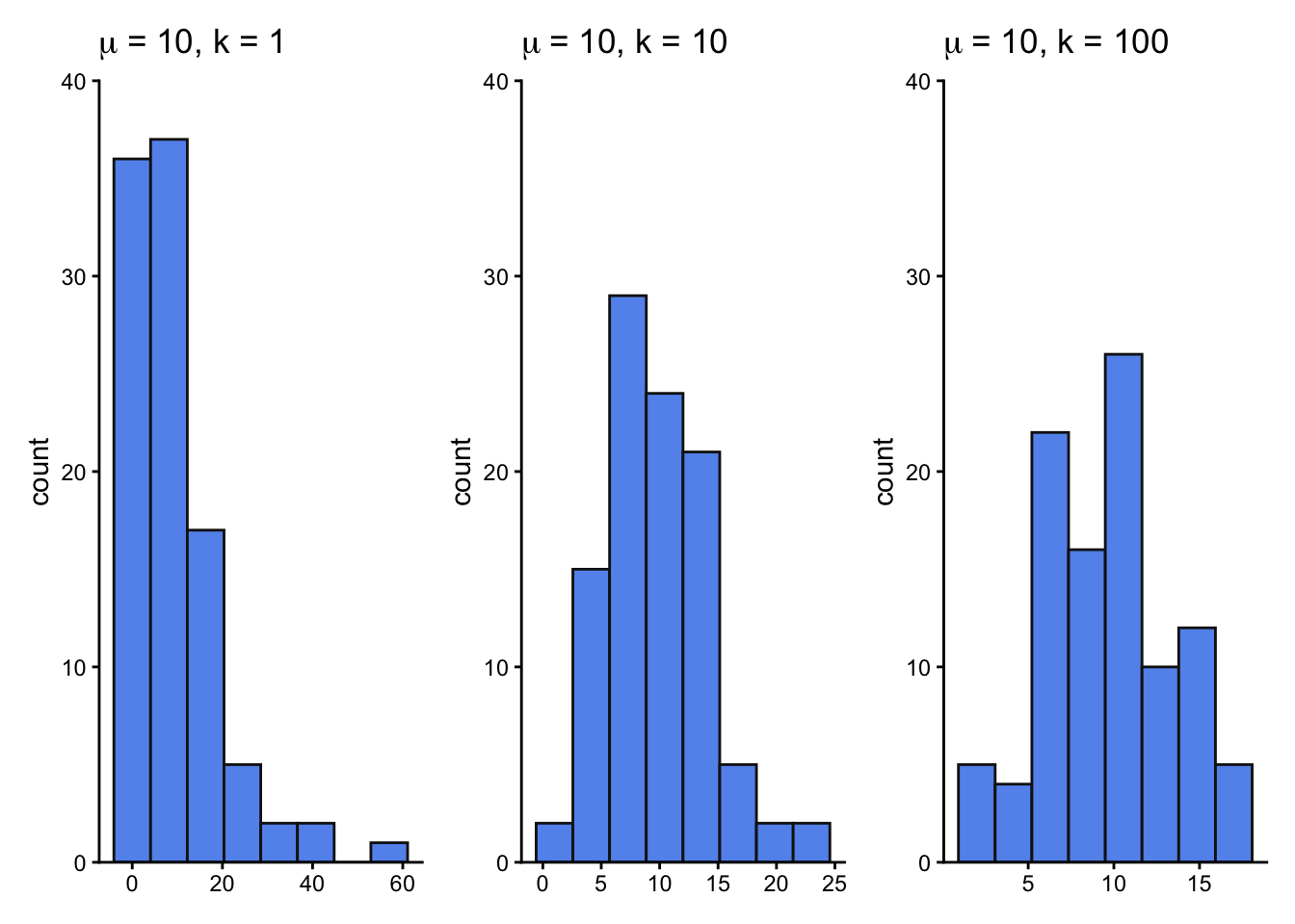
```{r nbinom-fig}
set.seed(666)
nbinom_df <- bind_cols(
size1 = rnbinom(mu = 10, size = 1, n = 100),
size10 = rnbinom(mu = 10, size = 10, n = 100),
size100 = rnbinom(mu = 10, size = 100, n = 100)
)
ggplot(data.frame(x = 1:20), aes(x)) +
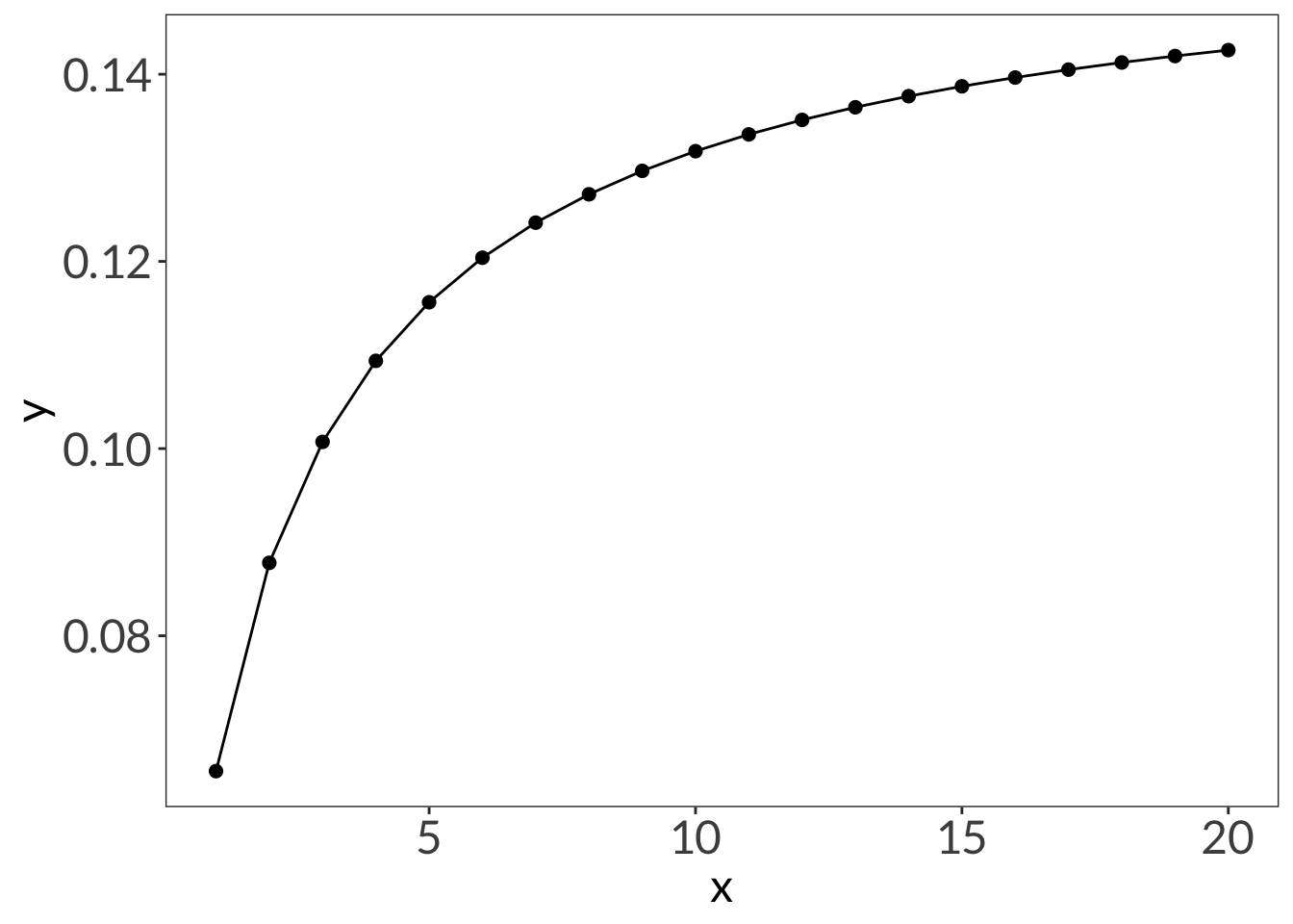
stat_function(geom = "point", n = 20, fun = dnbinom, args = list(mu = 4, x = 5), size = 2) +
stat_function(geom = "line", n = 20, fun = dnbinom, args = list(mu = 4, x = 5))
size1 <- ggplot(nbinom_df, aes(x = size1)) +
  geom_histogram(bins = 8, fill = "cornflowerblue", color = "grey8") +
  scale_y_continuous(expand = c(0, 0), limits = c(0, 40)) +
  theme_classic() +
  labs(title = expression(mu~"= 10, k = 1")) +
  theme(axis.title.x = element_blank())

size10 <- ggplot(nbinom_df, aes(x = size10)) +
  geom_histogram(bins = 8, fill = "cornflowerblue", color = "grey8") +
  scale_y_continuous(expand = c(0, 0), limits = c(0, 40)) +
  theme_classic() +
  labs(title = expression(mu~"= 10, k = 10")) +
  theme(axis.title.x = element_blank())

size100 <- ggplot(nbinom_df, aes(x = size100)) +
  geom_histogram(bins = 8, fill = "cornflowerblue", color = "grey8") +
  scale_y_continuous(expand = c(0, 0), limits = c(0, 40)) +
  theme_classic() +
  labs(title = expression(mu~"= 10, k = 100")) +
  theme(axis.title.x = element_blank())

size1 + size10 + size100
```
# poisson example
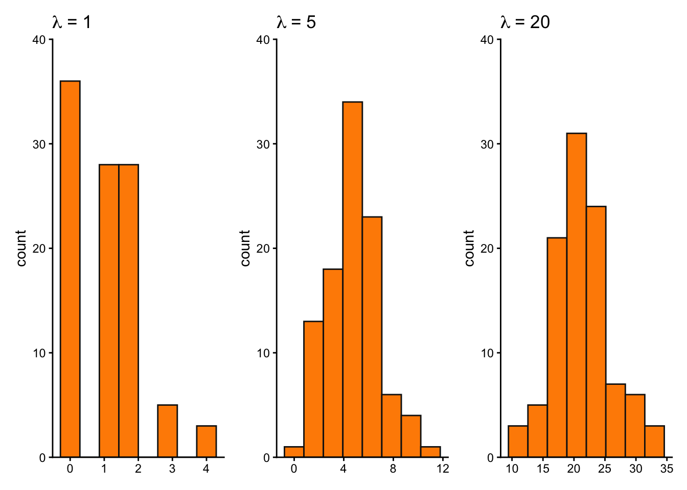
```{r pois-fig}
set.seed(666)
pois_df <- bind_cols(
  lambda1 = rpois(lambda = 1, n = 100),
  lambda5 = rpois(lambda = 5, n = 100),
  lambda20 = rpois(lambda = 20, n = 100)
)

lambda1 <- ggplot(pois_df, aes(x = lambda1)) +
  geom_histogram(bins = 8, fill = "darkorange", color = "grey8") +
  scale_y_continuous(expand = c(0, 0), limits = c(0, 40)) +
  theme_classic() +
  labs(title = expression(lambda~"= 1")) +
  theme(axis.title.x = element_blank())

lambda5 <- ggplot(pois_df, aes(x = lambda5)) +
  geom_histogram(bins = 8, fill = "darkorange", color = "grey8") +
  scale_y_continuous(expand = c(0, 0), limits = c(0, 40)) +
  theme_classic() +
  labs(title = expression(lambda~"= 5")) +
  theme(axis.title.x = element_blank())

lambda20 <- ggplot(pois_df, aes(x = lambda20)) +
  geom_histogram(bins = 8, fill = "darkorange", color = "grey8") +
  scale_y_continuous(expand = c(0, 0), limits = c(0, 40)) +
  theme_classic() +
  labs(title = expression(lambda~"= 20")) +
  theme(axis.title.x = element_blank())

lambda1 + lambda5 + lambda20
```
# bat example
## cleaning and displaying rows
```{r}
bats_clean <- bats |>
  mutate(date.x = mdy(date.x)) |>
  # create categories for disease load based on log-transformed values
  mutate(disease_load = case_when(
    logearlyloads < -3 ~ "low",
    between(logearlyloads, -3, -2) ~ "moderate",
    between(logearlyloads, -2, 0) ~ "high",
  ),
  # set factor levels for disease load: low --> high
  disease_load = fct_relevel(disease_load, "low", "moderate", "high")) |>
  # rename columns for clearer interpretation
  rename(recaptured_yn = EverRecapturedYN.x,
         temp = earlytemp) |>
  # select columns of interest
  select(recaptured_yn, temp, disease_load) |>
  filter(disease_load != "high")

slice_sample(
  bats_clean,
  n = 10
)
```
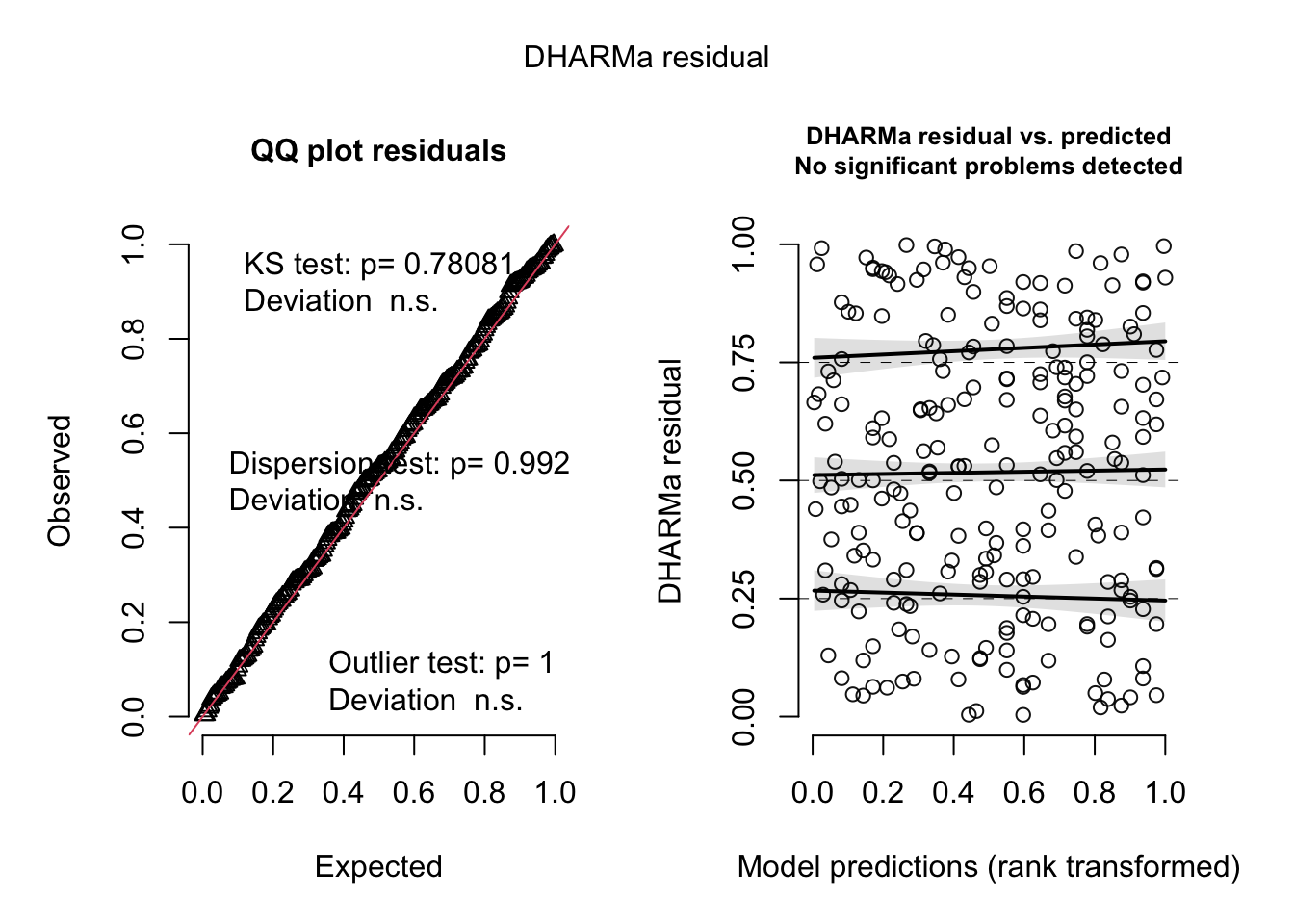
## fitting model and looking at diagnostics
```{r}
bat_mod <- glm(recaptured_yn ~ temp * disease_load,
               data = bats_clean,
               family = "binomial")

plot(
  simulateResiduals(bat_mod)
)
summary(bat_mod)
```
## generating predictions
```{r}
model_preds <- ggpredict(bat_mod,
                         terms = c("temp[all]",
                                   "disease_load")) |>
  rename(disease_load = group)

model_preds_with0 <- ggpredict(bat_mod,
                         terms = c("temp[0:12.3 by = 0.1]",
                                   "disease_load")) |>
  rename(disease_load = group)

ggpredict(bat_mod,
          terms = c("temp [0]",
                    "disease_load"))
ggpredict(bat_mod,
          terms = c("temp [4.8]",
                    "disease_load"))
ggpredict(bat_mod,
          terms = c("temp [8.0]",
                    "disease_load"))
ggpredict(bat_mod,
          terms = c("temp [12.3]",
                    "disease_load"))
```
## generating effects
```{r}
emtrends(bat_mod,
         specs = "disease_load",
         var = "temp")
# moderate
```
## plotting
```{r}
#| fig-height: 6
#| fig-width: 10
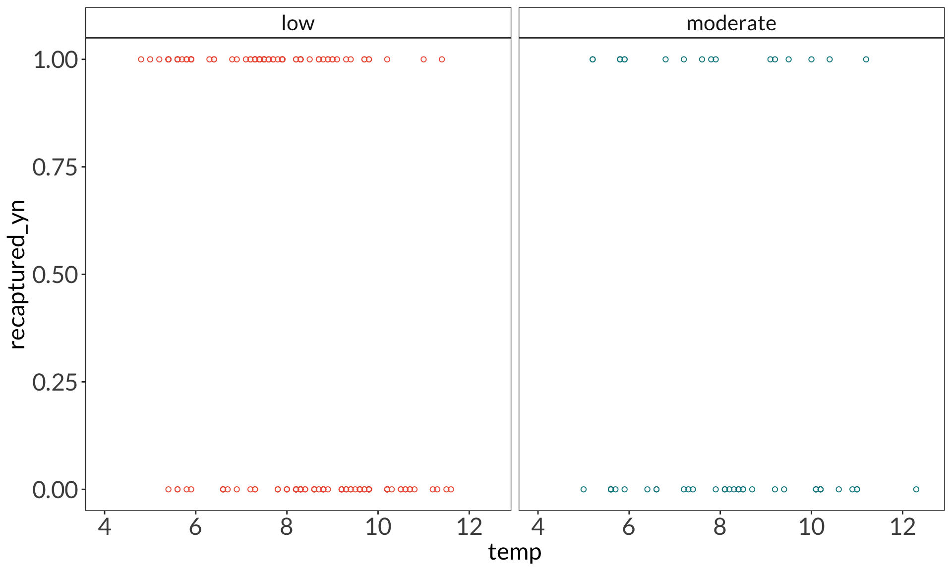
ggplot(data = bats_clean,
       aes(x = temp,
           y = recaptured_yn)) +
  geom_point(aes(color = disease_load),
             shape = 21) +
  scale_color_manual(values = c(
    "low" = "tomato2",
    "moderate" = "turquoise4"
  )) +
  scale_x_continuous(limits = c(4, 12.5),
                     breaks = c(4, 6, 8, 10, 12)) +
  facet_wrap(~ disease_load) +
  theme(legend.position = "none")
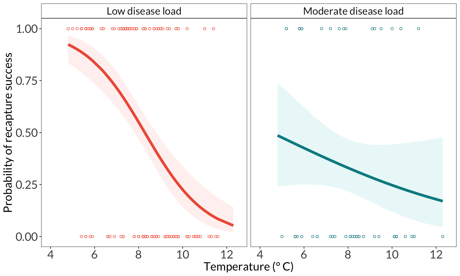
ggplot(data = bats_clean,
       aes(x = temp,
           y = recaptured_yn)) +
  geom_point(aes(color = disease_load),
             shape = 21) +
  geom_line(data = model_preds,
            aes(x = x,
                y = predicted,
                color = disease_load),
            linewidth = 2) +
  geom_ribbon(data = model_preds,
              aes(x = x,
                  y = predicted,
                  ymin = conf.low,
                  ymax = conf.high,
                  fill = disease_load),
              alpha = 0.1) +
  facet_wrap(~ disease_load,
             labeller = labeller(
               disease_load = c(low = "Low disease load",
                                moderate = "Moderate disease load")
             )) +
  scale_color_manual(values = c(
    "low" = "tomato2",
    "moderate" = "turquoise4"
  )) +
  scale_x_continuous(limits = c(4, 12.5),
                     breaks = c(4, 6, 8, 10, 12)) +
  labs(x = "Temperature (\U00B0 C)",
       y = "Probability of recapture success") +
  theme(legend.position = "none")
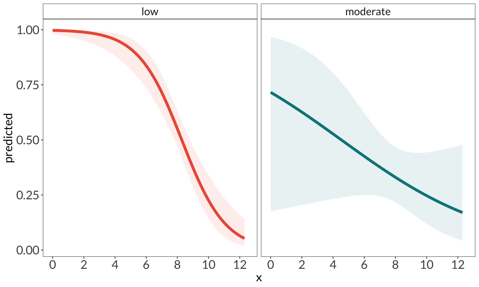
ggplot(data = model_preds_with0,
       aes(x = x,
           y = predicted)) +
  geom_ribbon(aes(x = x,
                  y = predicted,
                  ymin = conf.low,
                  ymax = conf.high,
                  fill = disease_load),
              alpha = 0.1) +
  geom_line(aes(color = disease_load),
            linewidth = 2) +
  scale_color_manual(values = c(
    "low" = "tomato2",
    "moderate" = "turquoise4"
  )) +
  scale_fill_manual(values = c(
    "low" = "tomato2",
    "moderate" = "turquoise4"
  )) +
  facet_wrap(~ disease_load) +
  scale_x_continuous(limits = c(0, 12.5),
                     breaks = c(0, 2, 4, 6, 8, 10, 12)) +
  theme(legend.position = "none")
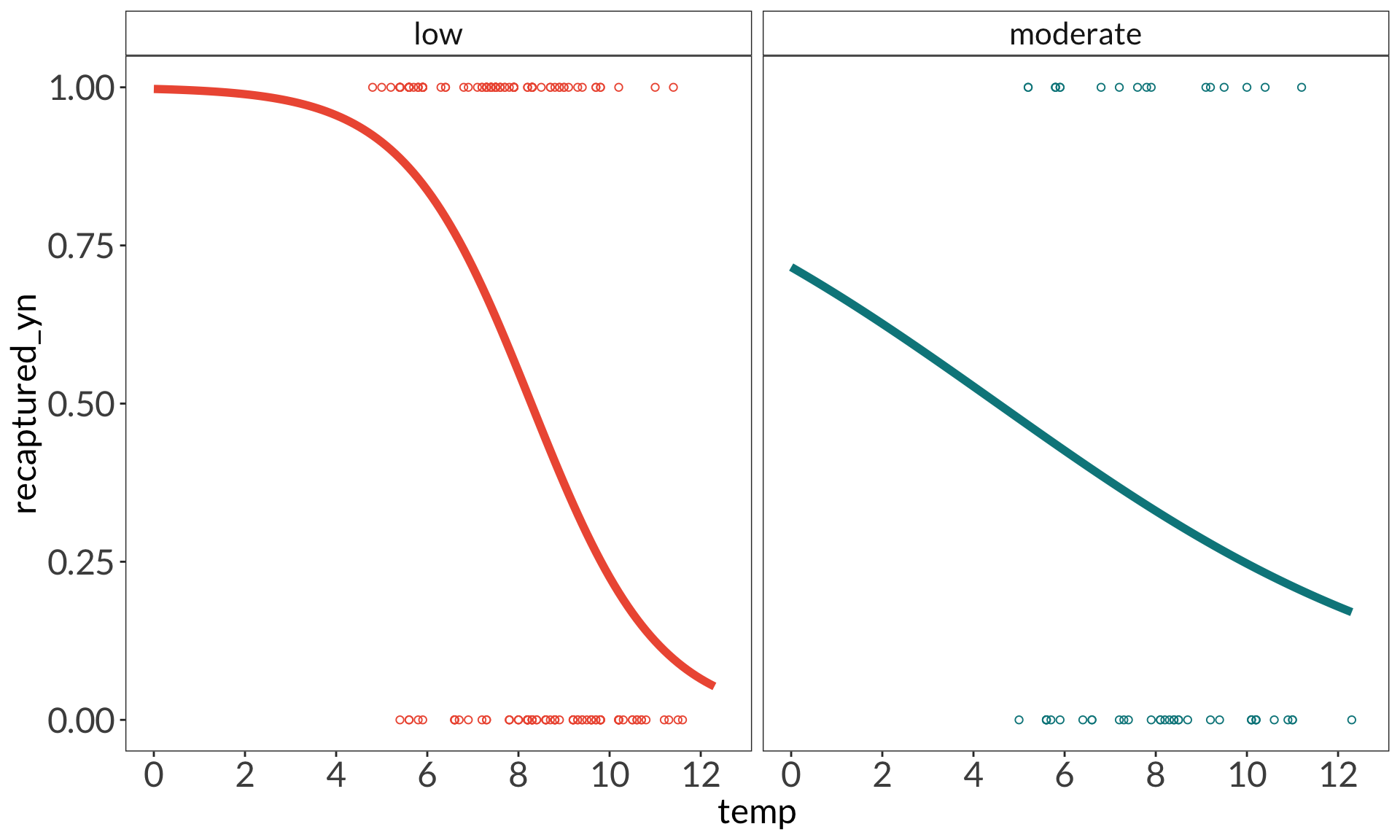
ggplot(data = model_preds_with0,
       aes(x = x,
           y = predicted)) +
  geom_point(data = bats_clean,
             aes(x = temp,
                 y = recaptured_yn,
                 color = disease_load),
             shape = 21) +
  geom_line(aes(color = disease_load),
            linewidth = 2) +
  scale_color_manual(values = c(
    "low" = "tomato2",
    "moderate" = "turquoise4"
  )) +
  scale_fill_manual(values = c(
    "low" = "tomato2",
    "moderate" = "turquoise4"
  )) +
  facet_wrap(~ disease_load) +
  scale_x_continuous(limits = c(0, 12.5),
                     breaks = c(0, 2, 4, 6, 8, 10, 12)) +
  theme(legend.position = "none")
as_flextable(bat_mod)
```