Code

# cleaning
library(tidyverse)
library(readxl)
library(here)
library(janitor)

# visualization
theme_set(theme_classic() +
            theme(panel.grid = element_blank(),
                  axis.text = element_text(size = 18),
                  axis.title = element_text(size = 18),
                  text = element_text(family = "Lato")))
library(patchwork)
library(ggeffects)
library(flextable)
library(GGally)

# data
library(palmerpenguins)

# analysis
library(car)
library(performance)
library(broom)
library(DHARMa)
library(MuMIn)
library(gtsummary)
library(emmeans)

drought_exp <- read_xlsx(
  # file path
  here("data", "Valliere_etal_EcoApps_Data.xlsx"),
  # specifying which sheet you want to read in
  sheet = "First Harvest"
)

multiple linear regression equation

\[ \begin{align} y &= \beta_0 + \beta_1x_1 + \beta_2x_2 + ... \beta_kx_k + \epsilon \end{align} \]

formulas

sum of squares for linear regression

regression (or model)

\[ SS_{reg} = \sum_{i = 1}^{n}(\hat{y} - \bar{y})^2 \]

error

\[ SS_{err} = \sum_{i = 1}^{n}(y_i - \hat{y})^2 \]

total

\[ SS_{tot} = \sum_{i = 1}^n(y_i - \bar{y}) \]

mean square

regression

\[ MS_{reg} = \frac{SS_{reg}}{1} \]

error

\[ MS_{err} = \frac{SS_{err}}{n - 2} \]

F-statistic

\[ F = \frac{MS_{reg}}{MS_{err}} \]

soil example

Code

set.seed(666)
# sample size
n <- 64

soil_df <- tibble(
  # compaction
  force_mpa = round(rnorm(n = n, mean = 0.7, sd = 0.03), 3),
  # root length
  root_mm = round(rnorm(n = n, mean = -1, sd = 0.02)*force_mpa, 3) + 5,
  # soil salinity
  salinity = round(rnorm(n = n, mean = 3, sd = 0.3)*force_mpa, 3)
) 

ggplot(data = soil_df,
       aes(x = force_mpa,
           y = root_mm)) +
  geom_point()

Code

ggplot(data = soil_df,
       aes(x = force_mpa,
           y = salinity)) +
  geom_point()

Code

soil_lm <- lm(
  root_mm ~ force_mpa,
  data = soil_df
)

par(mfrow = c(2, 2))
plot(soil_lm)

Code

summary(soil_lm)


Call:
lm(formula = root_mm ~ force_mpa, data = soil_df)

Residuals:
      Min        1Q    Median        3Q       Max 
-0.033749 -0.009088  0.000251  0.008962  0.028832 

Coefficients:
            Estimate Std. Error t value Pr(>|t|)    
(Intercept)   4.9569     0.0357   138.9   <2e-16 ***
force_mpa    -0.9400     0.0511   -18.4   <2e-16 ***
---
Signif. codes:  0 '***' 0.001 '**' 0.01 '*' 0.05 '.' 0.1 ' ' 1

Residual standard error: 0.01338 on 62 degrees of freedom
Multiple R-squared:  0.8451,    Adjusted R-squared:  0.8427 
F-statistic: 338.4 on 1 and 62 DF,  p-value: < 2.2e-16

Code

cor.test(soil_df$root_mm, soil_df$force_mpa,
         method = "pearson")


    Pearson's product-moment correlation

data:  soil_df$root_mm and soil_df$force_mpa
t = -18.395, df = 62, p-value < 2.2e-16
alternative hypothesis: true correlation is not equal to 0
95 percent confidence interval:
 -0.9503672 -0.8701422
sample estimates:
       cor 
-0.9193192

Code

cor.test(soil_df$root_mm, soil_df$force_mpa,
         method = "spearman")


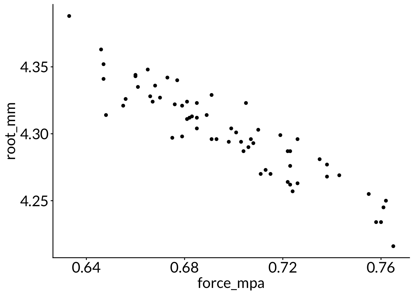
    Spearman's rank correlation rho

data:  soil_df$root_mm and soil_df$force_mpa
S = 83662, p-value < 2.2e-16
alternative hypothesis: true rho is not equal to 0
sample estimates:
       rho 
-0.9153354

Code

cor.test(soil_df$salinity, soil_df$force_mpa,
         method = "pearson")


    Pearson's product-moment correlation

data:  soil_df$salinity and soil_df$force_mpa
t = 2.5713, df = 62, p-value = 0.01254
alternative hypothesis: true correlation is not equal to 0
95 percent confidence interval:
 0.06995477 0.51680060
sample estimates:
      cor 
0.3104261

Code

cor.test(soil_df$salinity, soil_df$force_mpa,
         method = "spearman")


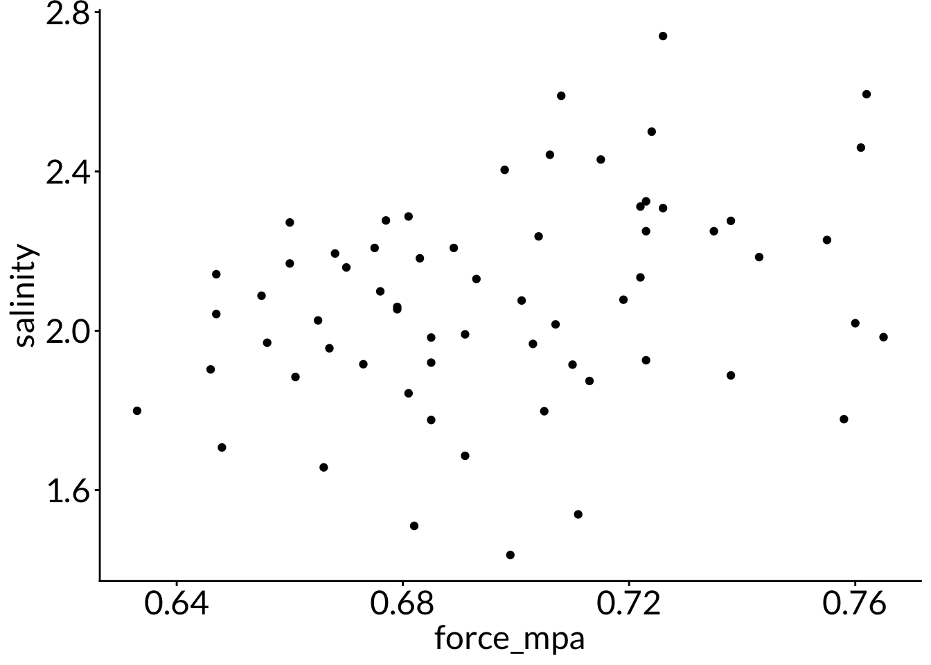
    Spearman's rank correlation rho

data:  soil_df$salinity and soil_df$force_mpa
S = 29861, p-value = 0.01087
alternative hypothesis: true rho is not equal to 0
sample estimates:
      rho 
0.3163656

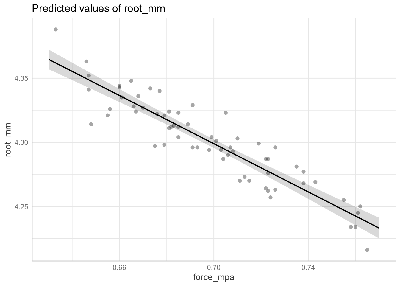
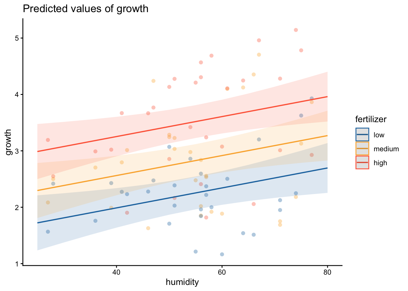
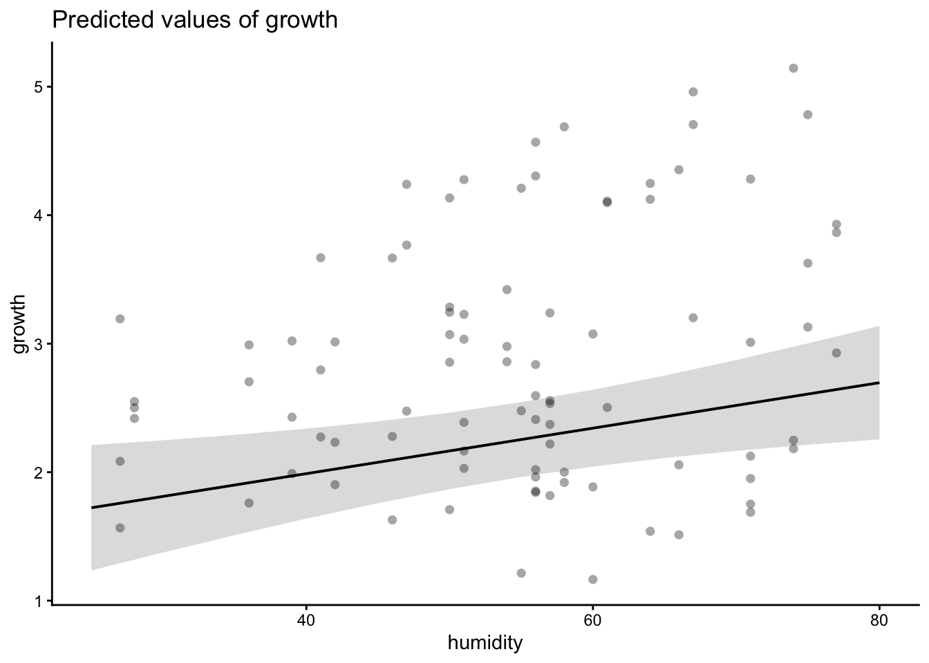
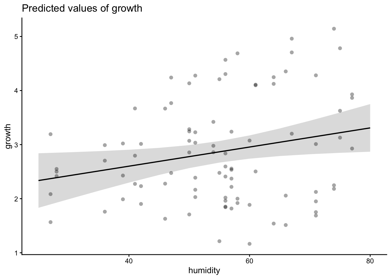
Code

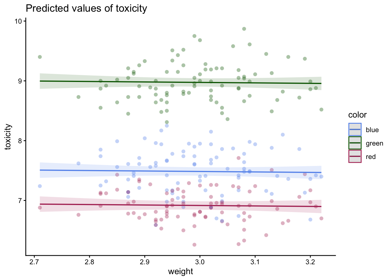
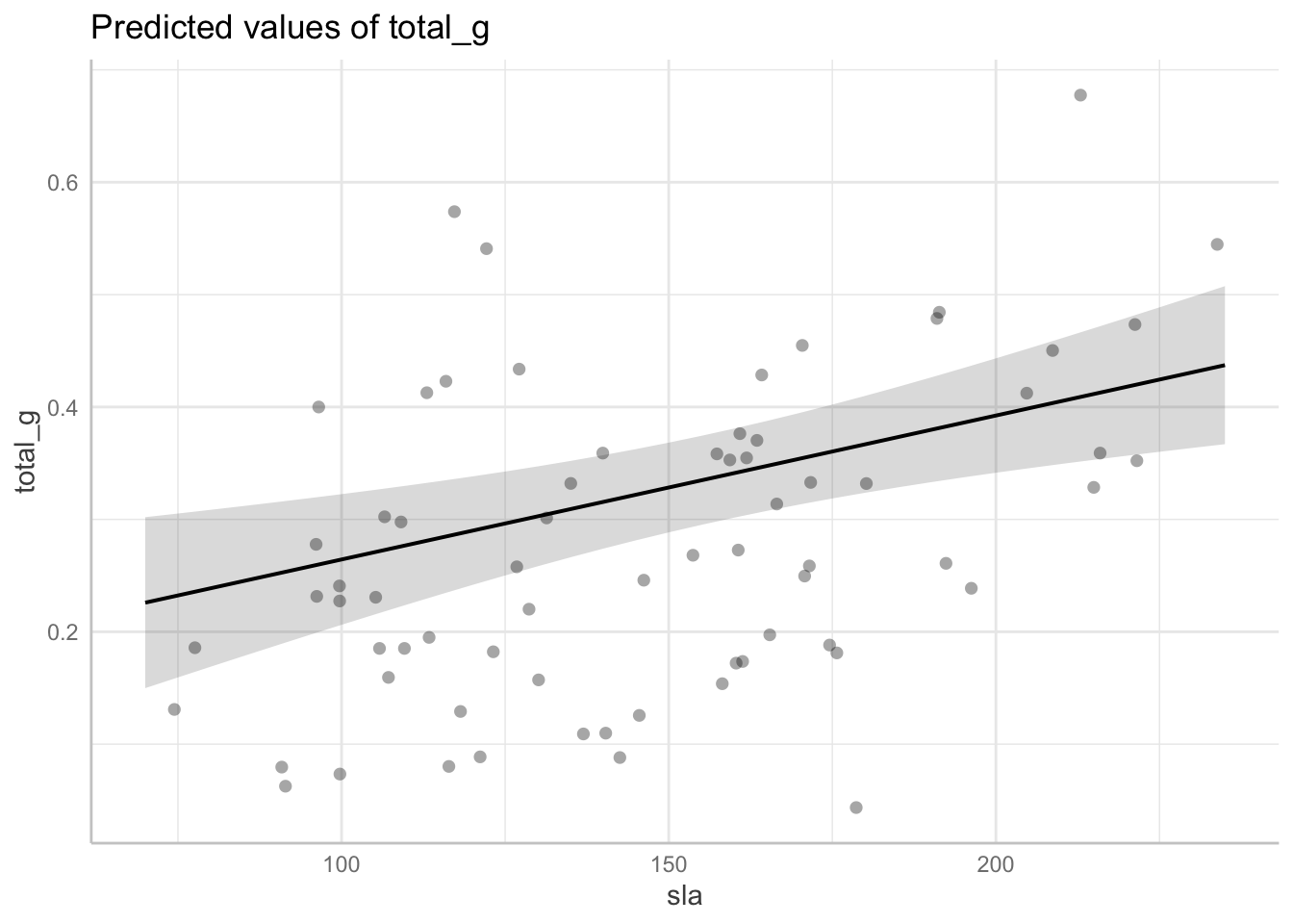
model_preds <- ggpredict(
  soil_lm,
  terms = "force_mpa [0.63:0.77 by = 0.01]"
) 

ggpredict(
  soil_lm,
  terms = "force_mpa [0.63:0.77 by = 0.01]") |> 
  plot(show_data = TRUE)

Code

flextable::as_flextable(soil_lm)

	Estimate	Standard Error	t value	Pr(>\|t\|)
(Intercept)	4.957	0.036	138.866	0.0000	***
force_mpa	-0.940	0.051	-18.395	0.0000	***
Signif. codes: 0 <= '*' < 0.001 < '' < 0.01 < '*' < 0.05

Residual standard error: 0.01338 on 62 degrees of freedom
Multiple R-squared: 0.8451, Adjusted R-squared: 0.8427
F-statistic: 338.4 on 62 and 1 DF, p-value: 0.0000

Code

flextable::as_flextable(soil_lm) %>% 
  set_formatter(
    # special function to represent p < 0.001
    values = list("p.value" = function(x){ 
      z <- scales::label_pvalue()(x)
      z[!is.finite(x)] <- ""
      z
    })
  )

	Estimate	Standard Error	t value	Pr(>\|t\|)
(Intercept)	4.957	0.036	138.866	<0.001	***
force_mpa	-0.940	0.051	-18.395	<0.001	***
Signif. codes: 0 <= '*' < 0.001 < '' < 0.01 < '*' < 0.05

Residual standard error: 0.01338 on 62 degrees of freedom
Multiple R-squared: 0.8451, Adjusted R-squared: 0.8427
F-statistic: 338.4 on 62 and 1 DF, p-value: 0.0000

plant example

Code

set.seed(666)
# sample size
n <- 64
plant_df <- tibble(
  # predictor variables
  temperature = round(rnorm(n = n, mean = 28, sd = 1), digits = 1),
  light = round(rnorm(n = n, mean = 1, sd = 0.2), digits = 1),
  ph = rnorm(n = n, mean = 7, sd = 0.01),
  
  # response: growth in cm/week
  growth = light*rnorm(n = n, mean = 0.3, sd = 0.1) + temperature/round(rnorm(n = n, mean = 5, sd = 0.1))
) 

ggplot(data = plant_df,
       aes(x = temperature,
           y = growth)) +
  geom_point()

Code

ggplot(data = plant_df,
       aes(x = ph,
           y = light)) +
  geom_point()

Code

ggplot(data = plant_df,
       aes(x = light,
           y = growth)) +
  geom_point()

Code

plant_lm <- lm(growth ~ temperature + ph + light,
               data = plant_df)
simulateResiduals(plant_lm) %>% plot()

Code

summary(plant_lm)


Call:
lm(formula = growth ~ temperature + ph + light, data = plant_df)

Residuals:
     Min       1Q   Median       3Q      Max 
-0.23209 -0.06571  0.01010  0.06173  0.19950 

Coefficients:
            Estimate Std. Error t value Pr(>|t|)    
(Intercept) -6.67140    6.80194  -0.981    0.331    
temperature  0.19626    0.01058  18.558  < 2e-16 ***
ph           0.96241    0.96806   0.994    0.324    
light        0.35196    0.05939   5.926 1.63e-07 ***
---
Signif. codes:  0 '***' 0.001 '**' 0.01 '*' 0.05 '.' 0.1 ' ' 1

Residual standard error: 0.0911 on 60 degrees of freedom
Multiple R-squared:  0.8759,    Adjusted R-squared:  0.8696 
F-statistic: 141.1 on 3 and 60 DF,  p-value: < 2.2e-16

Code

ggpredict(plant_lm,
          terms = c("temperature")) %>% 
  plot(show_data = TRUE)

Code

ggpredict(plant_lm,
          terms = c("ph")) %>% 
  plot(show_data = TRUE)

Code

ggpredict(plant_lm,
          terms = c("light")) %>% 
  plot(show_data = TRUE)

Code

plant_model <- lm(growth ~ light + temperature, 
                  data = plant_df)

Code

simulateResiduals(plant_model,
                  plot = TRUE)

Object of Class DHARMa with simulated residuals based on 250 simulations with refit = FALSE . See ?DHARMa::simulateResiduals for help. 
 
Scaled residual values: 0 0.756 0.792 0.816 0.06 0.132 0.408 0.708 0.988 0.892 0.452 0.876 0.644 0.512 0.984 0.904 0.936 0.56 0.58 0.724 ...

Code

check_model(plant_model)

Code

pairs(plant_df, upper.panel = NULL)

Code

ggpairs(plant_df)

Code

cor(plant_df)

            temperature       light          ph      growth
temperature  1.00000000  0.15540780 -0.06657697  0.89551840
light        0.15540780  1.00000000 -0.04769987  0.40397013
ph          -0.06657697 -0.04769987  1.00000000 -0.02466729
growth       0.89551840  0.40397013 -0.02466729  1.00000000

Code

vif(plant_model)

      light temperature 
   1.024749    1.024749

Code

summary(plant_model)


Call:
lm(formula = growth ~ light + temperature, data = plant_df)

Residuals:
      Min        1Q    Median        3Q       Max 
-0.227058 -0.071297  0.006266  0.063745  0.197573 

Coefficients:
            Estimate Std. Error t value Pr(>|t|)    
(Intercept)  0.08464    0.29166   0.290    0.773    
light        0.34972    0.05934   5.894 1.76e-07 ***
temperature  0.19563    0.01056  18.534  < 2e-16 ***
---
Signif. codes:  0 '***' 0.001 '**' 0.01 '*' 0.05 '.' 0.1 ' ' 1

Residual standard error: 0.09109 on 61 degrees of freedom
Multiple R-squared:  0.8738,    Adjusted R-squared:  0.8697 
F-statistic: 211.2 on 2 and 61 DF,  p-value: < 2.2e-16

Code

# anova(plant_model)

For example, temperature F-value:

Code

2.85039/0.0083

[1] 343.4205

\[ \begin{align} F &= \frac{2.85039}{0.00830} \\ &= 343.4205 \end{align} \]

dummy variable examples

Code

tibble(
  herbivores = sample(x = c("absent", "present"), size = 10, replace = TRUE, prob = c(0.5, 0.5))
)

# A tibble: 10 × 1
   herbivores
   <chr>     
 1 present   
 2 present   
 3 absent    
 4 present   
 5 absent    
 6 absent    
 7 absent    
 8 absent    
 9 absent    
10 present

Code

df <- tibble(
  fertilizer = sample(x = c("low", "medium", "high"), size = 10, replace = TRUE, prob = c(0.3, 0.3, 0.3))
) |> 
  mutate(fertilizer = as_factor(fertilizer),
         fertilizer = fct_relevel(fertilizer, "low", "medium", "high"))

str(df)

tibble [10 × 1] (S3: tbl_df/tbl/data.frame)
 $ fertilizer: Factor w/ 3 levels "low","medium",..: 2 2 3 1 2 3 1 1 2 2

Code

df <- tibble(
  year = sample(x = c("1st", "2nd", "3rd", "4th", "5th"), size = 20, replace = TRUE, prob = c(0.2, 0.2, 0.2, 0.2, 0.2))
) %>% 
  mutate(year = as_factor(year),
         year = fct_relevel(year, "1st", "2nd", "3rd", "4th", "5th"))

df

# A tibble: 20 × 1
   year 
   <fct>
 1 3rd  
 2 2nd  
 3 3rd  
 4 4th  
 5 3rd  
 6 5th  
 7 2nd  
 8 3rd  
 9 4th  
10 1st  
11 5th  
12 5th  
13 4th  
14 5th  
15 4th  
16 4th  
17 4th  
18 1st  
19 5th  
20 3rd

Code

str(df)

tibble [20 × 1] (S3: tbl_df/tbl/data.frame)
 $ year: Factor w/ 5 levels "1st","2nd","3rd",..: 3 2 3 4 3 5 2 3 4 1 ...

plant growth dummy variable

Code

# humidity units: %
# plant growth: cm / week

low_col <- "#2176ae"
medium_col <- "#fbb13c"
high_col <- "#fe6847"

n <- 30
set.seed(10)
plant_df <- tibble(
  humidity = round(rnorm(n = n, mean = 60, sd = 15), 0),
  low = humidity*rnorm(n = n, mean = 0.025, sd = 0.012) + 1,
  medium = humidity*rnorm(n = n, mean = 0.025, sd = 0.015) + 1.5,
  high = humidity*rnorm(n = n, mean = 0.025, sd = 0.017) + 2
) %>% 
  pivot_longer(cols = low:high,
               names_to = "fertilizer", 
               values_to = "growth") %>% 
  mutate(fertilizer = fct_relevel(fertilizer, "low", "medium", "high"))

# gives you a random sample
sample_n(plant_df, 10)

# A tibble: 10 × 3
   humidity fertilizer growth
      <dbl> <fct>       <dbl>
 1       71 high         3.01
 2       42 high         1.90
 3       58 medium       1.92
 4       50 low          3.07
 5       56 low          1.96
 6       61 low          2.50
 7       47 medium       4.24
 8       54 low          2.86
 9       77 low          3.93
10       39 medium       1.99

Code

# look at the structure
str(plant_df)

tibble [90 × 3] (S3: tbl_df/tbl/data.frame)
 $ humidity  : num [1:90] 60 60 60 57 57 57 39 39 39 51 ...
 $ fertilizer: Factor w/ 3 levels "low","medium",..: 1 2 3 1 2 3 1 2 3 1 ...
 $ growth    : num [1:90] 1.17 1.89 3.08 2.37 2.53 ...

Code

ggplot(data = plant_df,
       aes(x = humidity,
           y = growth)) +
  geom_point()

Code

ggplot(data = plant_df,
       aes(x = fertilizer,
           y = growth,
           color = fertilizer)) +
  geom_jitter(width = 0.2,
              height = 0,
              alpha = 0.3) +
  stat_summary(fun.data = mean_cl_normal,
               geom = "pointrange",
               size = 1,
               linewidth = 1) +
  scale_color_manual(values = c(low_col, medium_col, high_col)) +
  theme(legend.position = "none")

Code

plant_df %>% 
  group_by(fertilizer) %>% 
  summarize(mean = mean(growth))

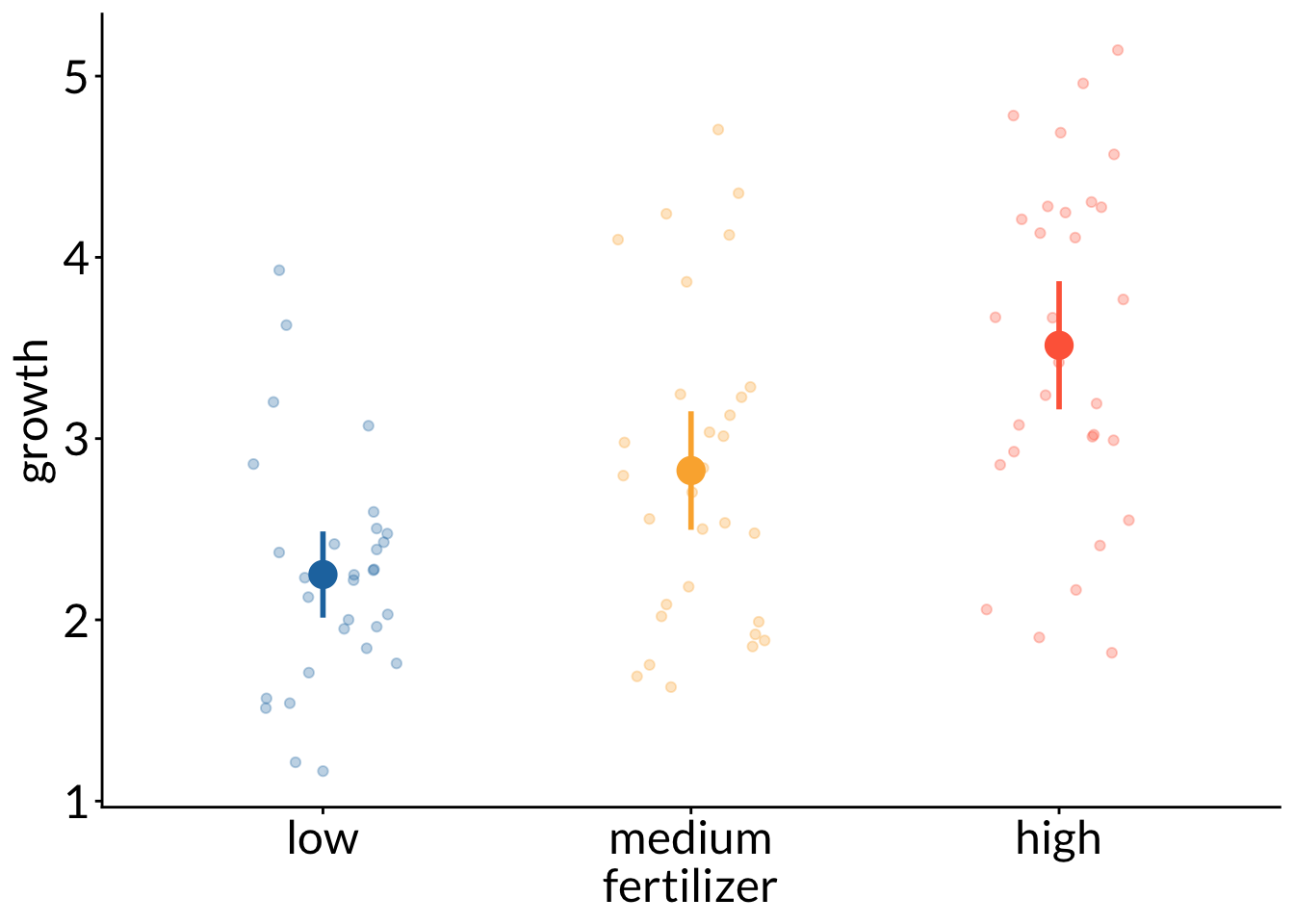
# A tibble: 3 × 2
  fertilizer  mean
  <fct>      <dbl>
1 low         2.25
2 medium      2.82
3 high        3.51

Code

plant_df %>% 
  summarize(mean = mean(growth))

# A tibble: 1 × 1
   mean
  <dbl>
1  2.86

Code

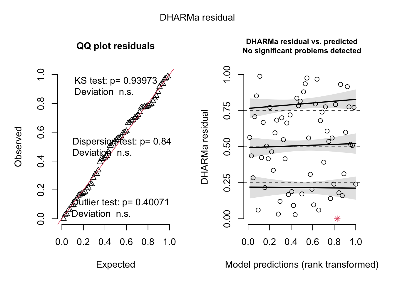
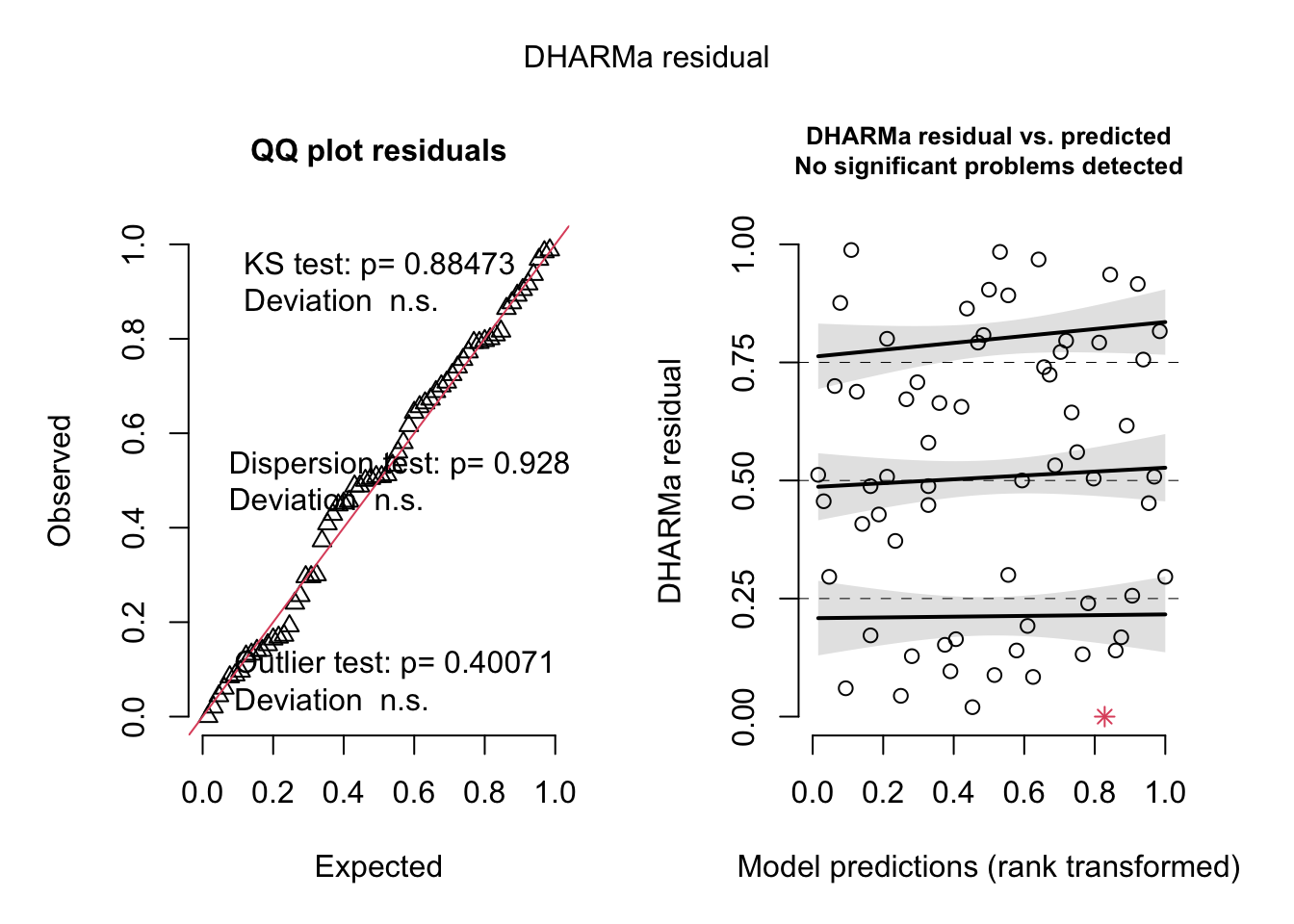
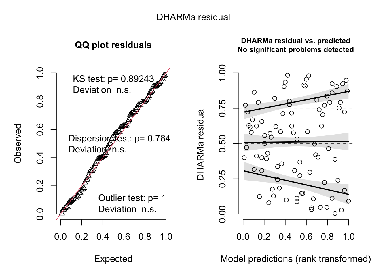
plant_lm <- lm(growth ~ humidity + fertilizer,
               data = plant_df)

# am i broken because i can't look at anything other than dharma residuals
simulateResiduals(plant_lm) %>% plot()

Code

par(mfrow = c(2, 2))
plot(plant_lm)

Code

ggpredict(plant_lm,
          terms = c("humidity",
                    "fertilizer")) %>% 
  plot(show_data = TRUE) +
  scale_color_manual(values = c(low_col, medium_col, high_col)) +
  scale_fill_manual(values = c(low_col, medium_col, high_col)) +
  theme_classic()

Code

ggpredict(plant_lm,
          terms = c("humidity")) %>% 
  plot(show_data = TRUE) +
  theme_classic()

Code

ggpredict(lm(growth ~ humidity, data = plant_df),
          terms = "humidity") %>% 
  plot(show_data = TRUE) +
  theme_classic()

Code

summary(plant_lm)


Call:
lm(formula = growth ~ humidity + fertilizer, data = plant_df)

Residuals:
    Min      1Q  Median      3Q     Max 
-1.7361 -0.5220  0.1129  0.5353  1.6649 

Coefficients:
                 Estimate Std. Error t value Pr(>|t|)    
(Intercept)      1.280788   0.390802   3.277  0.00151 ** 
humidity         0.017697   0.006615   2.675  0.00894 ** 
fertilizermedium 0.573791   0.207205   2.769  0.00688 ** 
fertilizerhigh   1.264891   0.207205   6.105 2.88e-08 ***
---
Signif. codes:  0 '***' 0.001 '**' 0.01 '*' 0.05 '.' 0.1 ' ' 1

Residual standard error: 0.8025 on 86 degrees of freedom
Multiple R-squared:  0.3411,    Adjusted R-squared:  0.3182 
F-statistic: 14.84 on 3 and 86 DF,  p-value: 7.19e-08

Code

summary(lm(growth ~ humidity, data = plant_df))


Call:
lm(formula = growth ~ humidity, data = plant_df)

Residuals:
    Min      1Q  Median      3Q     Max 
-1.7902 -0.7698 -0.0693  0.5993  1.9402 

Coefficients:
            Estimate Std. Error t value Pr(>|t|)    
(Intercept) 1.893683   0.440513   4.299 4.42e-05 ***
humidity    0.017697   0.007833   2.259   0.0263 *  
---
Signif. codes:  0 '***' 0.001 '**' 0.01 '*' 0.05 '.' 0.1 ' ' 1

Residual standard error: 0.9502 on 88 degrees of freedom
Multiple R-squared:  0.05483,   Adjusted R-squared:  0.04409 
F-statistic: 5.105 on 1 and 88 DF,  p-value: 0.02633

Code

tbl_regression(plant_lm,
               label = list(humidity = "Humidity (%)",
                            fertilizer = "Fertilizer treatment")) |> 
  as_flex_table()

Characteristic	Beta	95% CI	p-value
Humidity (%)	0.02	0.00, 0.03	0.009
Fertilizer treatment
low	—	—
medium	0.57	0.16, 0.99	0.007
high	1.3	0.85, 1.7	<0.001
Abbreviation: CI = Confidence Interval

Code

flextable::as_flextable(plant_lm)

	Estimate	Standard Error	t value	Pr(>\|t\|)
(Intercept)	1.281	0.391	3.277	0.0015	**
humidity	0.018	0.007	2.675	0.0089	**
fertilizermedium	0.574	0.207	2.769	0.0069	**
fertilizerhigh	1.265	0.207	6.105	0.0000	***
Signif. codes: 0 <= '*' < 0.001 < '' < 0.01 < '*' < 0.05

Residual standard error: 0.8025 on 86 degrees of freedom
Multiple R-squared: 0.3411, Adjusted R-squared: 0.3182
F-statistic: 14.84 on 86 and 3 DF, p-value: 0.0000

frog example

generating data

Code

set.seed(666)
frog_n <- 87

frog_df <- tibble(
  weight = (round(rnorm(n = frog_n, mean = 3, sd = 0.1), 2)),
  blue = round(rnorm(n = frog_n, mean = 2.5, sd = 0.09)*(round(rnorm(n = frog_n, mean = 3, sd = 0.1), 2)), 2),
  green = round(rnorm(n = frog_n, mean = 3, sd = 0.05)*(round(rnorm(n = frog_n, mean = 3, sd = 0.1), 2)), 2),
  red = round(rnorm(n = frog_n, mean = 2.3, sd = 0.05)*(round(rnorm(n = frog_n, mean = 3, sd = 0.1), 2)), 2)
) %>% 
  pivot_longer(cols = blue:red,
               names_to = "color",
               values_to = "toxicity")

df <- cbind(
  # predictor variables
  # color = sample(x = c("blue", "green", "red"), size = frog_n, replace = TRUE, prob = c(0.3, 0.3, 0.3)),
  weight = (round(rnorm(n = frog_n, mean = 3, sd = 0.1), 2))
  #pattern = sample(x = c("striped", "spotted", "none"), size = frog_n, replace = TRUE, prob = c(0.3, 0.3, 0.3))
) %>%
  as_tibble() %>%
  mutate(toxicity = round(rnorm(n = frog_n, mean = 1.5, sd = 0.06)*weight, 3)) %>%
  mutate(color = case_when(
    between(toxicity, 2.5, 4.4) ~ "blue",
    between(toxicity, 4.4, 4.6) ~ "green",
    between(toxicity, 4.6, 5.5) ~ "red"
  )) %>% 
  mutate(toxicity = case_when(
    color == "blue" ~ round(rnorm(n = frog_n, mean = 2.5, sd = 0.09)*weight, 3),
    color == "green" ~ round(rnorm(n = frog_n, mean = 3, sd = 0.05)*weight, 3),
    color == "red" ~ round(rnorm(n = frog_n, mean = 2.3, sd = 0.05)*weight, 3)
  )) %>% 
  mutate(color = as_factor(color),
         color = fct_relevel(color, "red", "blue", "green"))


# df <- cbind(
#   color = sample(x = c("blue", "green", "red"), size = frog_n, replace = TRUE, prob = c(0.3, 0.3, 0.3))
# ) %>% 
#   as_tibble() %>% 
#   mutate(weight = (round(rnorm(n = frog_n, mean = 3.5, sd = 0.1), 2))) %>% 
#   mutate(toxicity = case_when(
#     color == "blue" ~ round(rnorm(n = frog_n, mean = 3, sd = 0.4)*weight, 2),
#     color == "green" ~ round(rnorm(n = frog_n, mean = 2, sd = 0.5)*weight, 2),
#     color == "red" ~ round(rnorm(n = frog_n, mean = 1, sd = 0.03)*weight, 2)
#   ))

plotting data

Code

blue_col <- "cornflowerblue"
green_col <- "darkgreen"
red_col <- "maroon"

striped_col <- "grey1"
spotted_col <- "grey50"
none_col <- "grey80"

ggplot(data = frog_df, aes(x = color, y = toxicity, color = color, fill = color)) +
  geom_jitter(width = 0.2, height = 0, alpha = 0.3) +
  scale_color_manual(values = c("blue" = blue_col, "green" = green_col, "red" = red_col)) +
  scale_fill_manual(values = c("blue" = blue_col, "green" = green_col, "red" = red_col)) +
  stat_summary(geom = "pointrange", 
               fun = mean, 
               fun.min = function(x) mean(x) - sd(x), 
               fun.max = function(x) mean(x) + sd(x), 
               shape = 21, 
               size = 1) +
 #  geom_point(position = position_jitter(width = 0.2, height = 0, seed = 666), alpha = 0.3) +
  labs(title = "Color") +
  theme(legend.position = "none",
        axis.title.x = element_blank(),
        text = element_text(size = 22))

Code

ggplot(data = frog_df, aes(x = weight, y = toxicity)) +
  geom_point() +
  # geom_smooth(method = "lm") +
  labs(title = "Weight") +
  theme(legend.position = "none",
        axis.title.x = element_blank(),
        text = element_text(size = 22))

Code

ggplot(data = frog_df, aes(x = weight, y = toxicity, color = color)) +
  geom_point() +
  scale_color_manual(values = c("blue" = blue_col, "green" = green_col, "red" = red_col)) +
  geom_smooth(method = "lm") +
  labs(title = "Weight")

Code

head(df, 10)

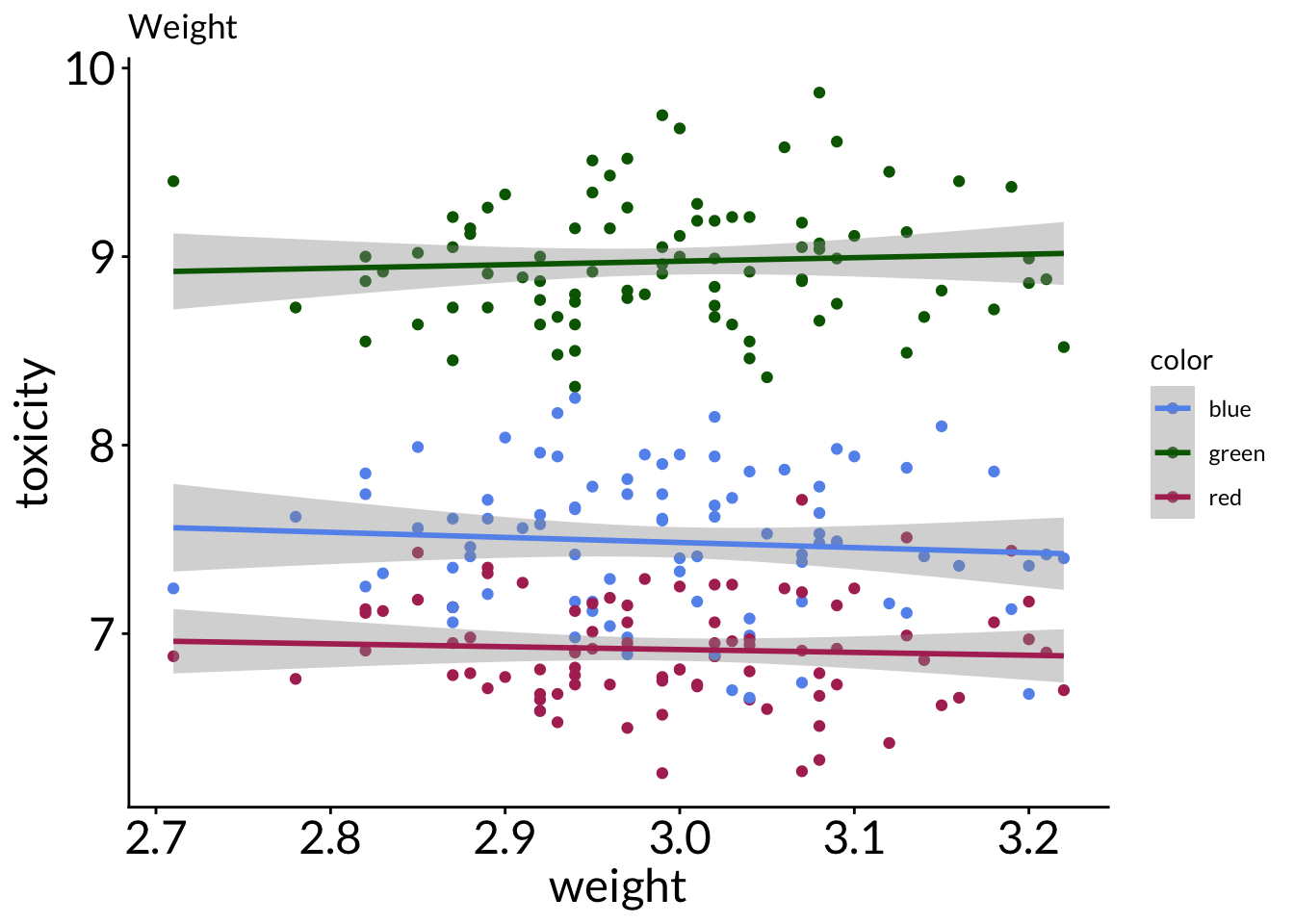
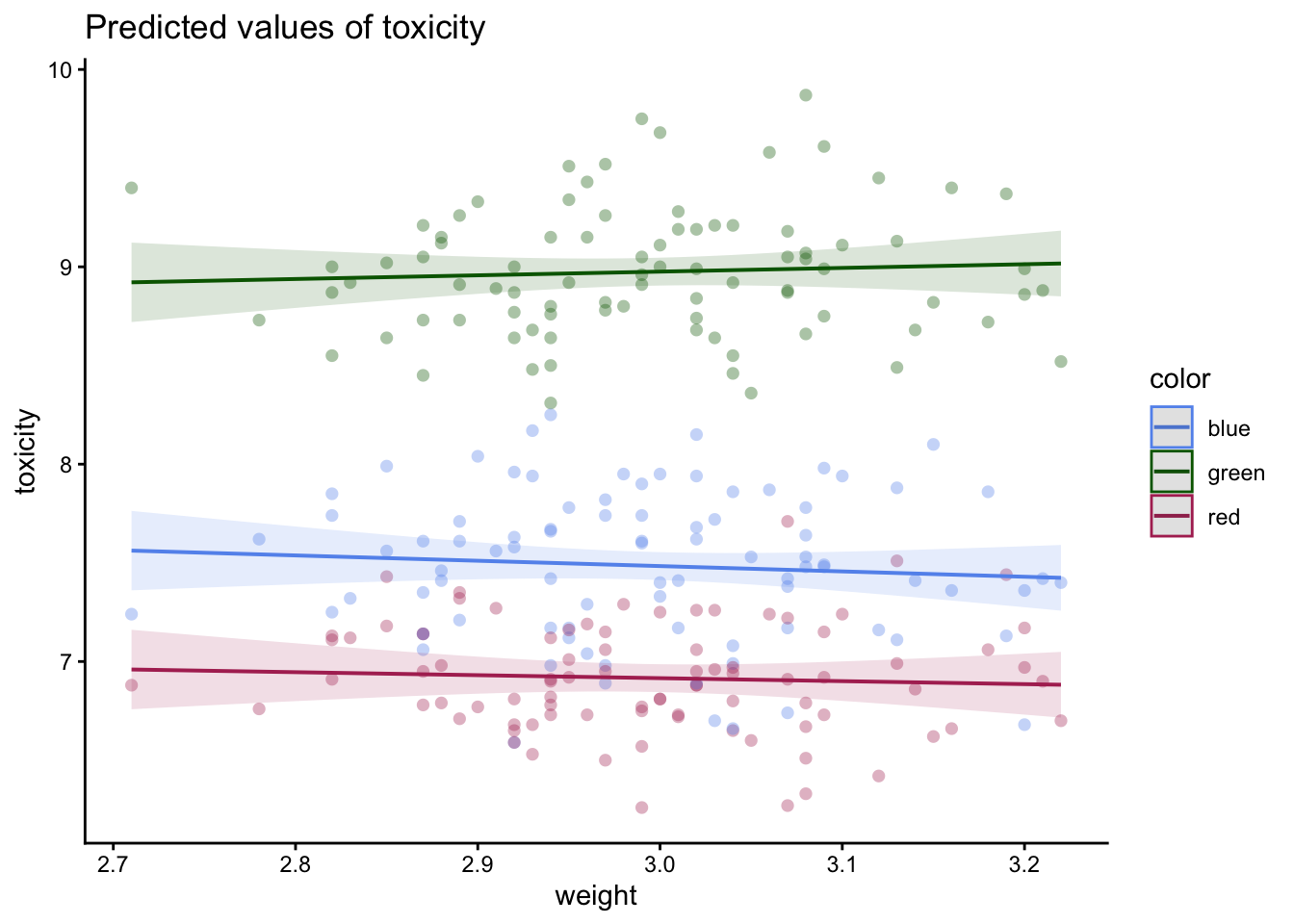
# A tibble: 10 × 3
   weight toxicity color
    <dbl>    <dbl> <fct>
 1   3.18     8.29 blue 
 2   3.02     9.24 green
 3   3.01     8.75 green
 4   3.07     7.24 red  
 5   2.98     7.47 blue 
 6   2.94     8.89 green
 7   2.95     7.26 blue 
 8   2.91     7.25 blue 
 9   2.95     6.61 red  
10   3.06     8.96 green

model

Code

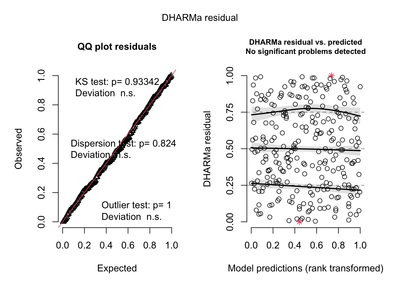
model1 <- lm(toxicity ~ weight + color, 
             data = frog_df)

model2 <- lm(toxicity ~ weight * color, 
             data = frog_df)

simulateResiduals(model1, plot = TRUE)

Object of Class DHARMa with simulated residuals based on 250 simulations with refit = FALSE . See ?DHARMa::simulateResiduals for help. 
 
Scaled residual values: 0.804 0.556 0.336 0.376 0.5 0.56 0.076 0.74 0.308 0.008 0.416 0.828 0.684 0.204 0.272 0.66 0.172 0.208 0.604 0.708 ...

Code

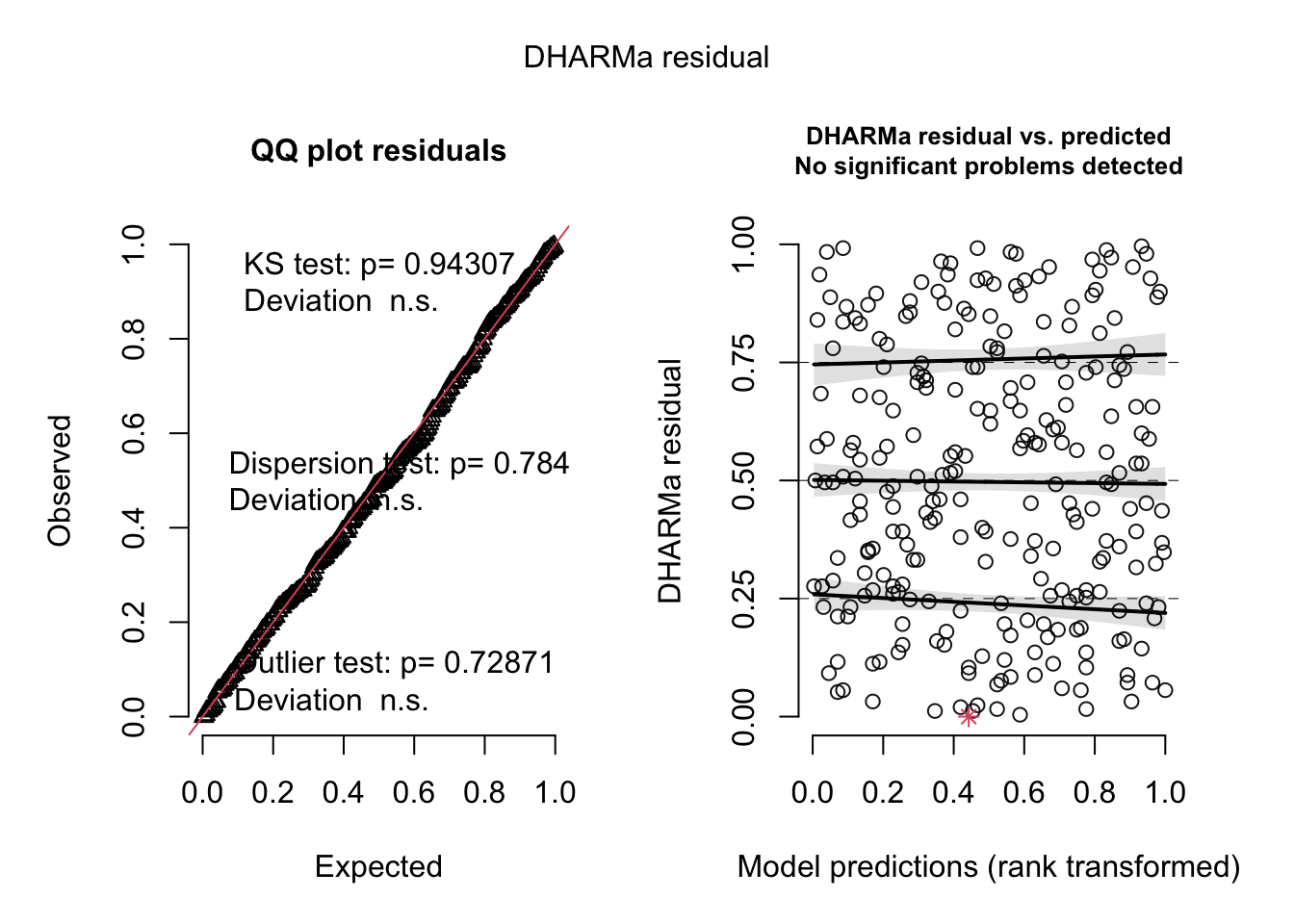
simulateResiduals(model2, plot = TRUE)

Object of Class DHARMa with simulated residuals based on 250 simulations with refit = FALSE . See ?DHARMa::simulateResiduals for help. 
 
Scaled residual values: 0.82 0.536 0.336 0.42 0.436 0.572 0.076 0.74 0.3 0.012 0.368 0.84 0.628 0.256 0.244 0.692 0.144 0.212 0.58 0.752 ...

Code

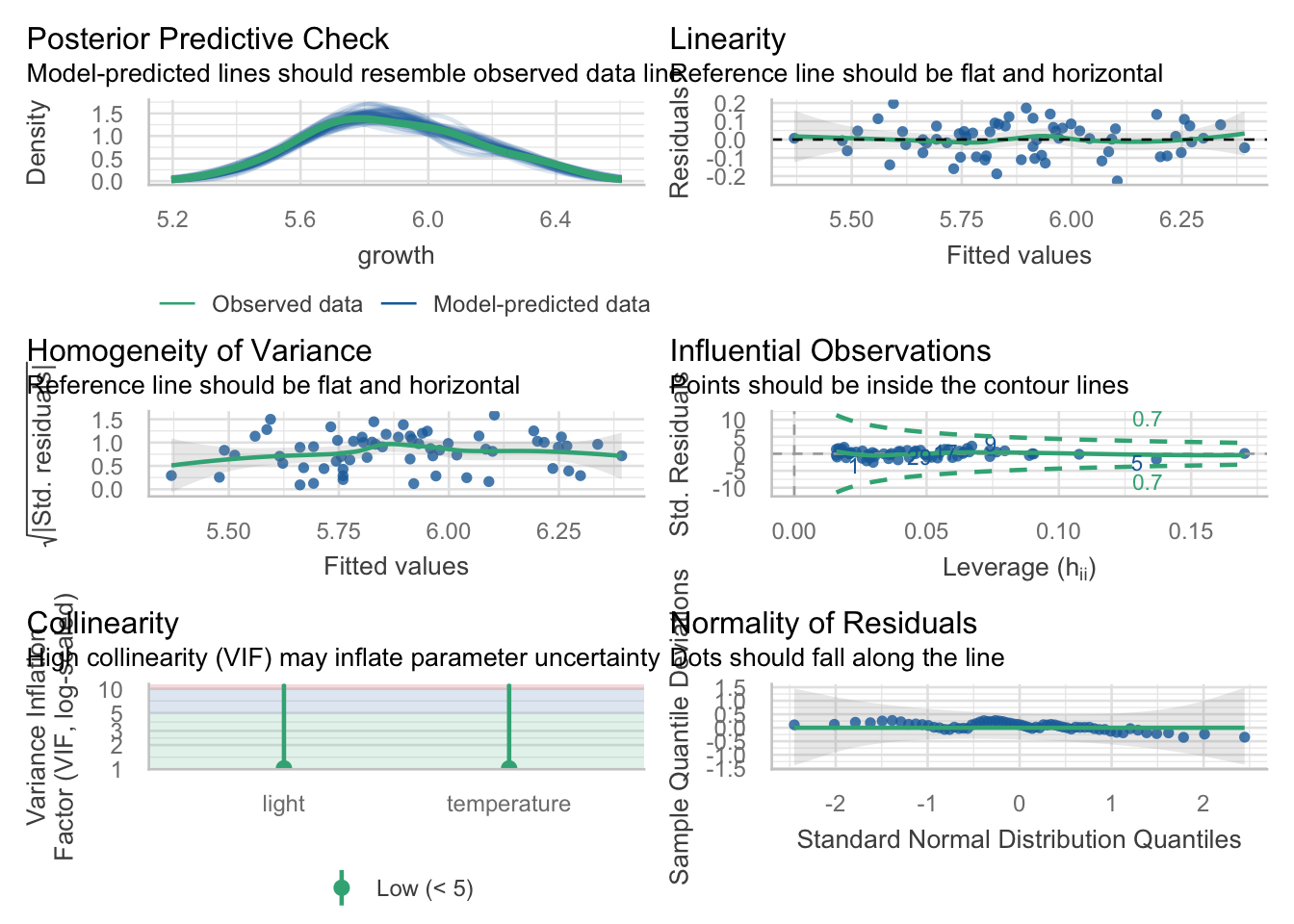
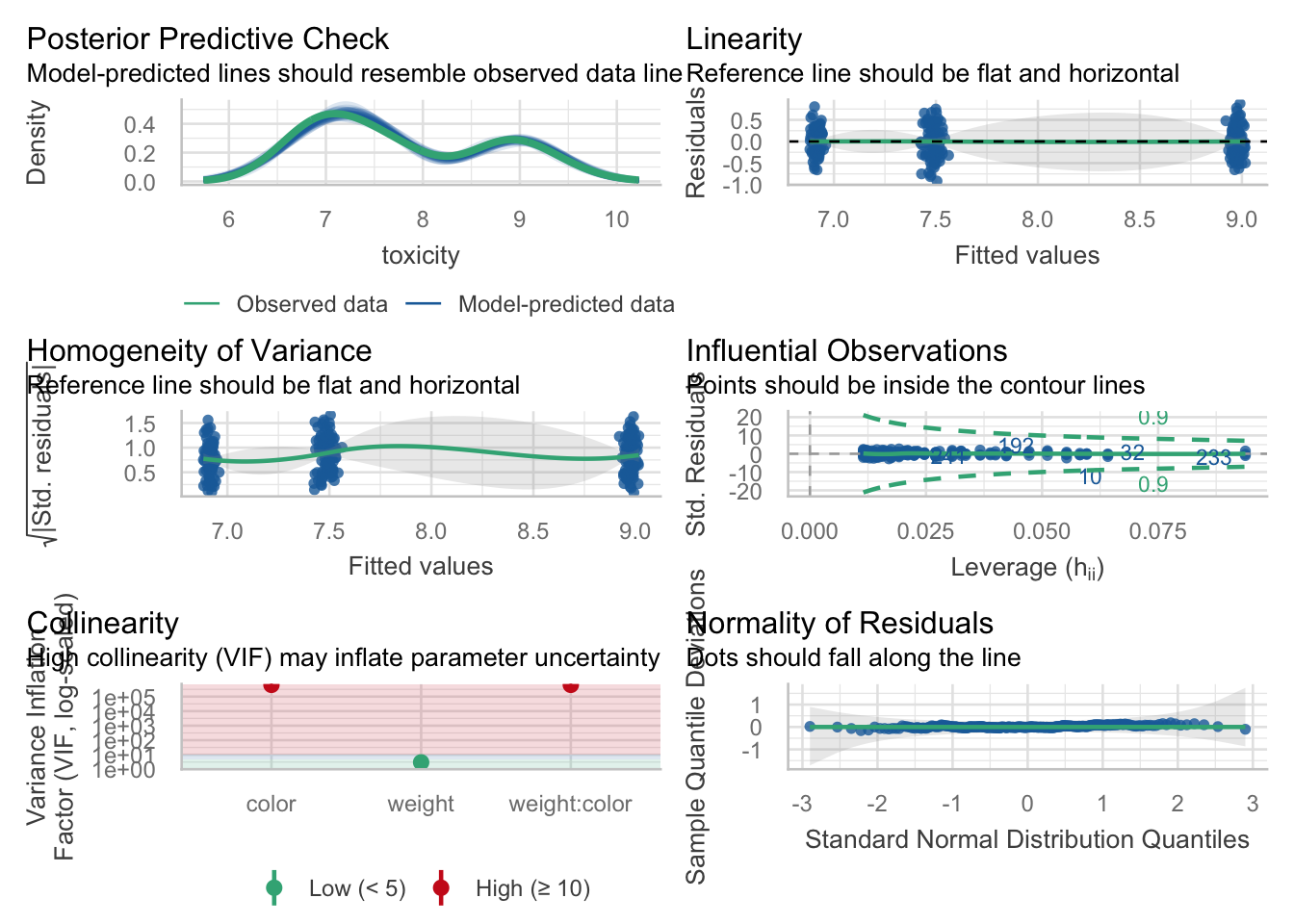
check_model(model2)

Code

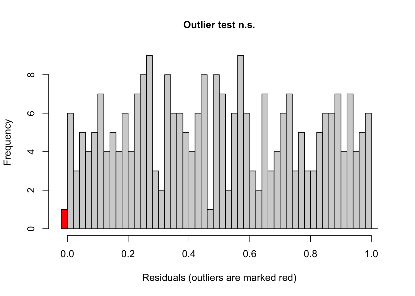
testOutliers(model2)


    DHARMa outlier test based on exact binomial test with approximate
    expectations

data:  model2
outliers at both margin(s) = 1, observations = 261, p-value = 0.7287
alternative hypothesis: true probability of success is not equal to 0.007968127
95 percent confidence interval:
 9.699839e-05 2.116127e-02
sample estimates:
frequency of outliers (expected: 0.00796812749003984 ) 
                                           0.003831418

diagnostics

Code

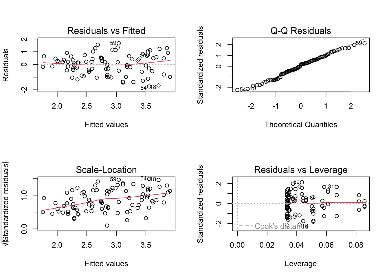
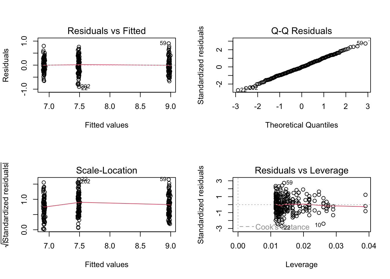
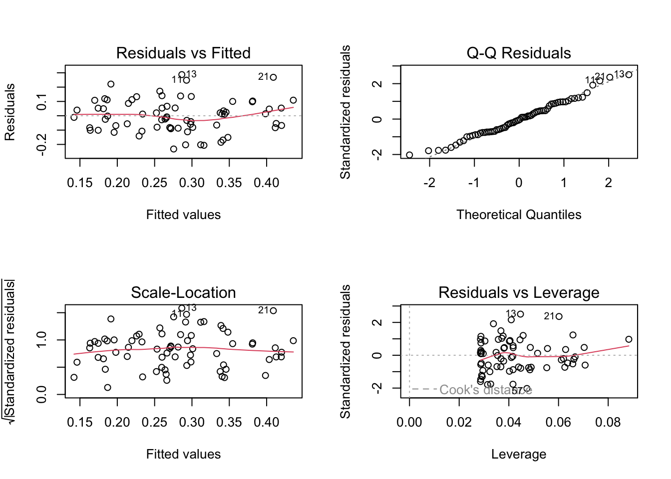
par(mfrow = c(2, 2))
plot(model1)

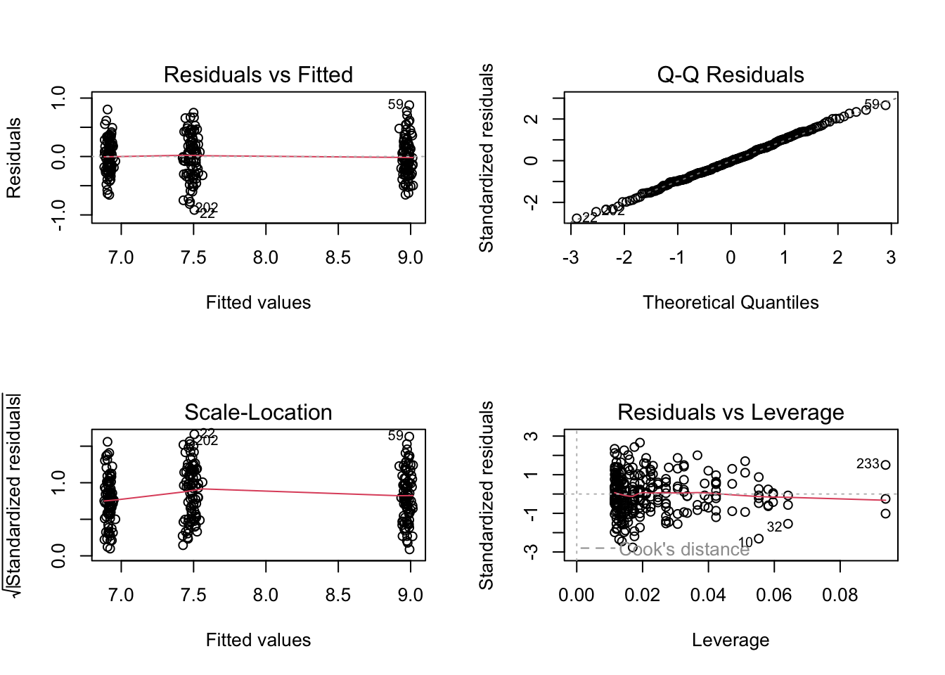
Code

plot(model2)

model summary

Code

summary(model1)


Call:
lm(formula = toxicity ~ weight + color, data = frog_df)

Residuals:
     Min       1Q   Median       3Q      Max 
-0.90113 -0.21865 -0.00068  0.22588  0.90229 

Coefficients:
            Estimate Std. Error t value Pr(>|t|)    
(Intercept)  7.71921    0.58381  13.222   <2e-16 ***
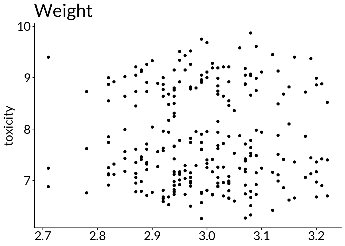
weight      -0.07811    0.19467  -0.401    0.689    
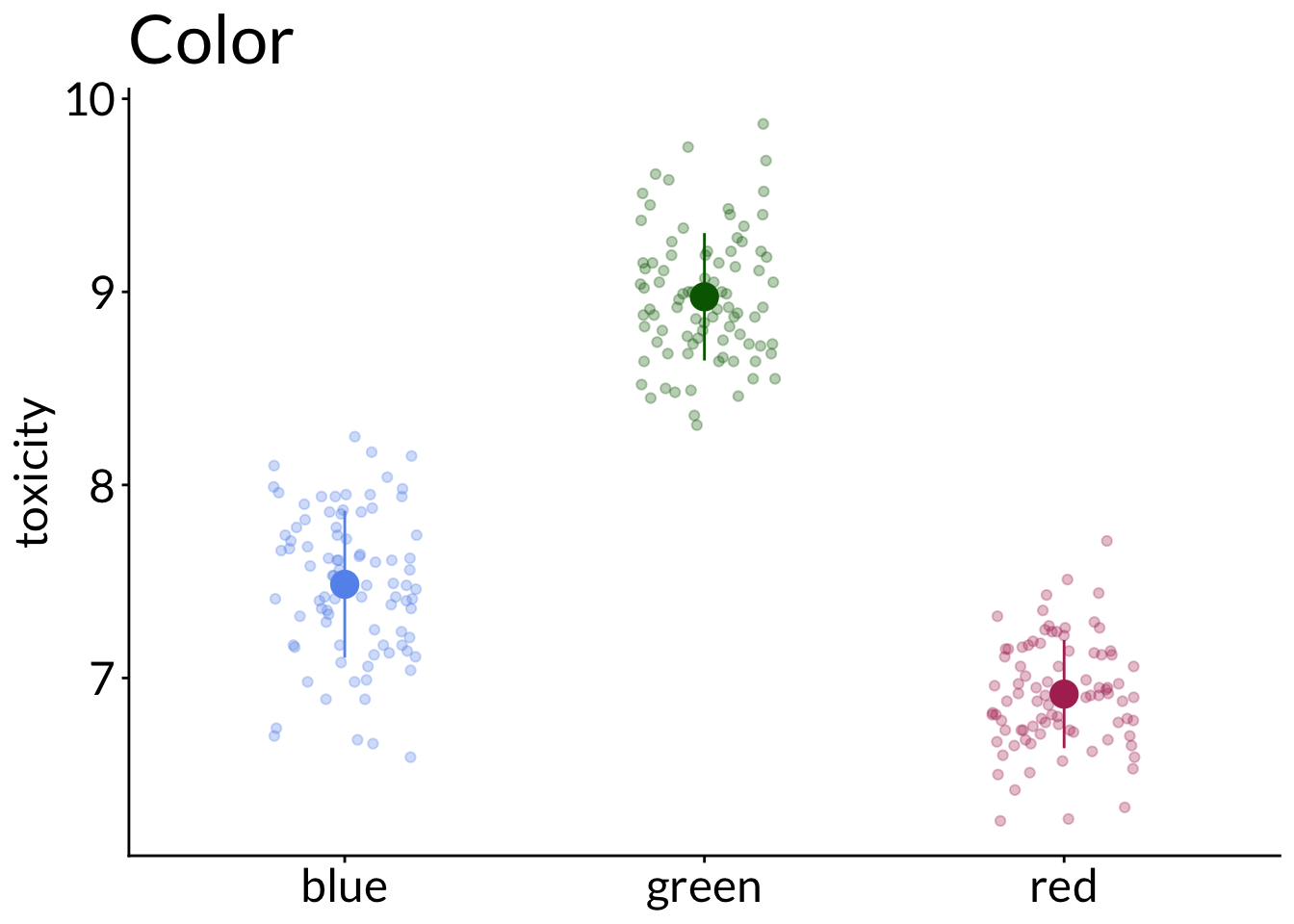
colorgreen   1.48908    0.05049  29.490   <2e-16 ***
colorred    -0.56874    0.05049 -11.263   <2e-16 ***
---
Signif. codes:  0 '***' 0.001 '**' 0.01 '*' 0.05 '.' 0.1 ' ' 1

Residual standard error: 0.333 on 257 degrees of freedom
Multiple R-squared:  0.8733,    Adjusted R-squared:  0.8718 
F-statistic: 590.6 on 3 and 257 DF,  p-value: < 2.2e-16

Code

summary(model2)


Call:
lm(formula = toxicity ~ weight * color, data = frog_df)

Residuals:
     Min       1Q   Median       3Q      Max 
-0.91522 -0.22141 -0.00686  0.21240  0.87930 

Coefficients:
                  Estimate Std. Error t value Pr(>|t|)    
(Intercept)         8.2941     1.0119   8.196 1.21e-14 ***
weight             -0.2702     0.3379  -0.800    0.425    
colorgreen          0.1204     1.4311   0.084    0.933    
colorred           -0.9248     1.4311  -0.646    0.519    
weight:colorgreen   0.4573     0.4778   0.957    0.339    
weight:colorred     0.1189     0.4778   0.249    0.804    
---
Signif. codes:  0 '***' 0.001 '**' 0.01 '*' 0.05 '.' 0.1 ' ' 1

Residual standard error: 0.3337 on 255 degrees of freedom
Multiple R-squared:  0.8738,    Adjusted R-squared:  0.8713 
F-statistic: 353.1 on 5 and 255 DF,  p-value: < 2.2e-16

Code

model.sel(model1, model2)

Model selection table 
       (Int) clr   wgh clr:wgh df  logLik  AICc delta
model1 7.719   + 0.832          5 -81.355 172.9   0.0
model2 8.294   + 0.168       +  7 -80.851 176.1   3.2
Models ranked by AICc(x)

Code

emmeans(model2,
        specs = c("weight", "color"))

 weight color emmean     SE  df lower.CL upper.CL
   2.99 blue    7.49 0.0358 255     7.41     7.56
   2.99 green   8.97 0.0358 255     8.90     9.04
   2.99 red     6.92 0.0358 255     6.85     6.99

Confidence level used: 0.95

Code

ggpredict(model1,
          terms = c("weight [2:4 by = 0.01]", 
                    "color")) %>% 
  plot(show_data = TRUE,
       limit_range = TRUE) +
  scale_color_manual(values = c("green" = green_col, 
                                "red" = red_col, 
                                "blue" = blue_col)) +
  scale_fill_manual(values = c("green" = green_col, 
                               "red" = red_col, 
                               "blue" = blue_col)) +
  theme_classic()

Code

ggpredict(model2,
          terms = c("weight [2:4 by = 0.01]", 
                    "color")) %>% 
  plot(show_data = TRUE,
       limit_range = TRUE) +
  scale_color_manual(values = c("green" = green_col, 
                                "red" = red_col, 
                                "blue" = blue_col)) +
  scale_fill_manual(values = c("green" = green_col, 
                               "red" = red_col, 
                               "blue" = blue_col)) +
  theme_classic()

\[ \hat{y}_h \pm t_{(1-\alpha/2, n-2)}*\sqrt{MSE*(\frac{1}{n}+\frac{(x_h-\bar{x})^2}{\sum(x_i-\bar{x})^2})} \]

\[ MSE = \frac{\sum(y_i-\hat{y})^2}{n} \]

Code

tidy(model2, conf.int = TRUE, conf.level = 0.95)

# A tibble: 6 × 7
  term              estimate std.error statistic  p.value conf.low conf.high
  <chr>                <dbl>     <dbl>     <dbl>    <dbl>    <dbl>     <dbl>
1 (Intercept)          8.29      1.01     8.20   1.21e-14    6.30     10.3  
2 weight              -0.270     0.338   -0.800  4.25e- 1   -0.936     0.395
3 colorgreen           0.120     1.43     0.0841 9.33e- 1   -2.70      2.94 
4 colorred            -0.925     1.43    -0.646  5.19e- 1   -3.74      1.89 
5 weight:colorgreen    0.457     0.478    0.957  3.39e- 1   -0.484     1.40 
6 weight:colorred      0.119     0.478    0.249  8.04e- 1   -0.822     1.06

Code

model_summary <- summary(model2)
c("lower" = model_summary$coef[2,1] - qt(0.975, df = model_summary$df[2]) * model_summary$coef[2, 2],
  "upper" = model_summary$coef[2,1] + qt(0.975, df = model_summary$df[2]) * model_summary$coef[2, 2])

     lower      upper 
-0.9355103  0.3951563

Confidence interval for a single coefficient: in words: estimate plus or minus the t-value at your confidence level * standard error

Valliere et al.

Code

drought_exp_clean <- drought_exp |> 
  clean_names() |> 
  mutate(water = case_when(
    water == "WW" ~ "Well watered",
    water == "DS" ~ "Drought stressed"
  )) |> 
  rename(treatment = water,
         species_name = species) |> 
  mutate(treatment = as_factor(treatment))


str(drought_exp_clean)

tibble [70 × 13] (S3: tbl_df/tbl/data.frame)
 $ species_name     : chr [1:70] "ENCCAL" "ENCCAL" "ENCCAL" "ENCCAL" ...
 $ treatment        : Factor w/ 2 levels "Well watered",..: 1 1 1 1 1 2 2 2 2 2 ...
 $ rep_number       : num [1:70] 1 2 3 4 5 1 2 3 4 5 ...
 $ height_cm        : num [1:70] 5.8 4.9 8.4 6.5 7.1 3.2 4.4 4.2 4.5 3.9 ...
 $ leaf_number      : num [1:70] 11 8 11 12 10 7 7 10 8 6 ...
 $ leaf_dry_weight_g: num [1:70] 0.0294 0.0185 0.0177 0.0178 0.0164 0.017 0.0193 0.0153 0.0159 0.0133 ...
 $ leaf_area_cm2    : num [1:70] 5.01 3.98 3.69 3.84 3.63 3.06 3.1 2.94 2.73 2.61 ...
 $ sla              : num [1:70] 170 215 209 216 222 ...
 $ total_la         : num [1:70] 55.1 31.8 40.6 46.1 36.3 ...
 $ shoot_g          : num [1:70] 0.253 0.164 0.241 0.213 0.232 ...
 $ root_g           : num [1:70] 0.202 0.165 0.209 0.146 0.12 ...
 $ total_g          : num [1:70] 0.455 0.329 0.45 0.359 0.352 ...
 $ r_s              : num [1:70] 0.8 1 0.9 0.7 0.5 0.8 1.2 3.1 0.9 1.2 ...

Code

pull(drought_exp_clean, treatment)

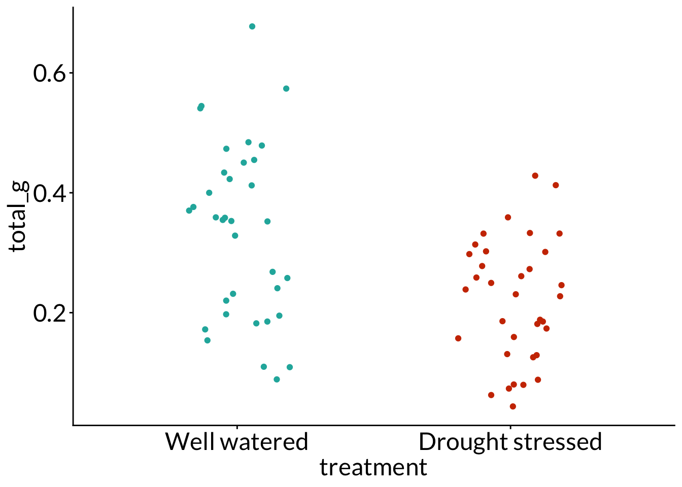
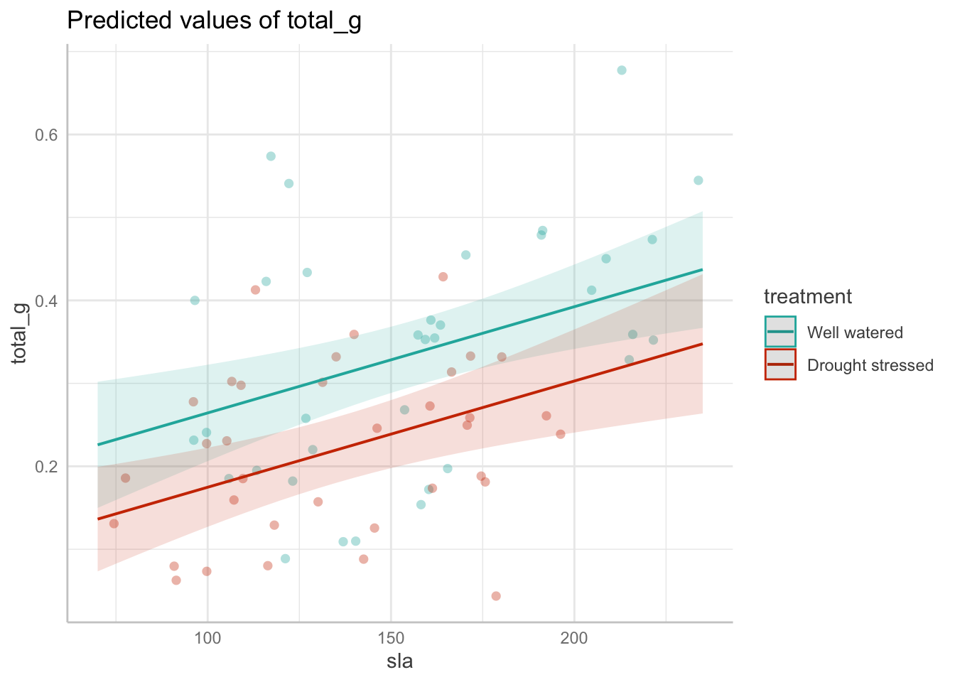
 [1] Well watered     Well watered     Well watered     Well watered    
 [5] Well watered     Drought stressed Drought stressed Drought stressed
 [9] Drought stressed Drought stressed Well watered     Well watered    
[13] Well watered     Well watered     Well watered     Drought stressed
[17] Drought stressed Drought stressed Drought stressed Drought stressed
[21] Well watered     Well watered     Well watered     Well watered    
[25] Well watered     Drought stressed Drought stressed Drought stressed
[29] Drought stressed Drought stressed Well watered     Well watered    
[33] Well watered     Well watered     Well watered     Drought stressed
[37] Drought stressed Drought stressed Drought stressed Drought stressed
[41] Well watered     Well watered     Well watered     Well watered    
[45] Well watered     Drought stressed Drought stressed Drought stressed
[49] Drought stressed Drought stressed Well watered     Well watered    
[53] Well watered     Well watered     Well watered     Drought stressed
[57] Drought stressed Drought stressed Drought stressed Drought stressed
[61] Well watered     Well watered     Well watered     Well watered    
[65] Well watered     Drought stressed Drought stressed Drought stressed
[69] Drought stressed Drought stressed
Levels: Well watered Drought stressed

Code

slice_sample(drought_exp_clean,
             n = 10)

# A tibble: 10 × 13
   species_name treatment     rep_number height_cm leaf_number leaf_dry_weight_g
   <chr>        <fct>              <dbl>     <dbl>       <dbl>             <dbl>
 1 SALLEU       Well watered           3       3.1           6            0.0343
 2 ENCCAL       Well watered           1       5.8          11            0.0294
 3 PENCEN       Drought stre…          2       1.9           6            0.0064
 4 SALLEU       Drought stre…          3       1.9           4            0.0304
 5 STIPUL       Drought stre…          4       9.7          16            0.0067
 6 GRICAM       Well watered           4       7.1           8            0.0451
 7 GRICAM       Drought stre…          5       4.3           6            0.0217
 8 SALLEU       Drought stre…          5       2.8           6            0.0296
 9 PENCEN       Drought stre…          4       2.1           5            0.0074
10 LOTSCO       Drought stre…          2       5.2          21            0.0033
# ℹ 7 more variables: leaf_area_cm2 <dbl>, sla <dbl>, total_la <dbl>,
#   shoot_g <dbl>, root_g <dbl>, total_g <dbl>, r_s <dbl>

Code

ggplot(data = drought_exp_clean,
       aes(x = sla,
           y = total_g)) +
  geom_point(color = "darkgreen")

Code

ggplot(data = drought_exp_clean,
       aes(x = reorder(species_name, -sla),
           y = sla,
           color = species_name)) +
  geom_jitter(height = 0,
              width = 0.2) +
  theme(legend.position = "none")

Code

ggplot(data = drought_exp_clean,
       aes(x = treatment,
           y = total_g,
           color = treatment)) +
  geom_jitter(height = 0,
              width = 0.2) +
  scale_color_manual(values = c(
    "Well watered" = "lightseagreen",
    "Drought stressed" = "orangered3"
  )) +
  theme(legend.position = "none")

Code

mod <- lm(
  total_g ~ sla + treatment,
  data = drought_exp_clean
)

model0 <- lm(
  total_g ~ 1,
  data = drought_exp_clean
)

model1 <- lm(
  total_g ~ sla + treatment + species_name,
  data = drought_exp_clean
)

model4 <- lm(
  total_g ~ treatment + species_name,
  data = drought_exp_clean
)

par(mfrow = c(2, 2))
plot(mod)

Code

summary(mod)


Call:
lm(formula = total_g ~ sla + treatment, data = drought_exp_clean)

Residuals:
      Min        1Q    Median        3Q       Max 
-0.231899 -0.082814 -0.004803  0.081373  0.287369 

Coefficients:
                            Estimate Std. Error t value Pr(>|t|)   
(Intercept)                0.1362657  0.0619544   2.199  0.03130 * 
sla                        0.0012807  0.0003736   3.428  0.00104 **
treatmentDrought stressed -0.0895679  0.0291549  -3.072  0.00307 **
---
Signif. codes:  0 '***' 0.001 '**' 0.01 '*' 0.05 '.' 0.1 ' ' 1

Residual standard error: 0.1173 on 67 degrees of freedom
Multiple R-squared:  0.3031,    Adjusted R-squared:  0.2823 
F-statistic: 14.57 on 2 and 67 DF,  p-value: 5.566e-06

Code

ggpredict(
  mod,
  terms = c("sla")
) |> 
  plot(show_data = TRUE)

Code

preds <- ggpredict(
  mod,
  terms = c("sla", "treatment")
) |> 
  rename(treatment = group)

ggpredict(
  mod,
  terms = c("sla[0]", "treatment"))

# Predicted values of total_g

treatment: Well watered

sla | Predicted |     95% CI
----------------------------
  0 |      0.14 | 0.01, 0.26

treatment: Drought stressed

sla | Predicted |      95% CI
-----------------------------
  0 |      0.05 | -0.06, 0.16

Code

ggpredict(
  mod,
  terms = c("sla", "treatment")
) |> 
  plot(show_data = TRUE) +
  scale_color_manual(values = c(
    "Well watered" = "lightseagreen",
    "Drought stressed" = "orangered3"
  )) +
  scale_fill_manual(values = c(
    "Well watered" = "lightseagreen",
    "Drought stressed" = "orangered3"
  ))

Code

as_flextable(mod)

	Estimate	Standard Error	t value	Pr(>\|t\|)
(Intercept)	0.136	0.062	2.199	0.0313	*
sla	0.001	0.000	3.428	0.0010	**
treatmentDrought stressed	-0.090	0.029	-3.072	0.0031	**
Signif. codes: 0 <= '*' < 0.001 < '' < 0.01 < '*' < 0.05

Residual standard error: 0.1173 on 67 degrees of freedom
Multiple R-squared: 0.3031, Adjusted R-squared: 0.2823
F-statistic: 14.57 on 67 and 2 DF, p-value: 0.0000

Code

tbl_regression(mod)

Characteristic	Beta	95% CI	p-value
sla	0.00	0.00, 0.00	0.001
treatment
Well watered	—	—
Drought stressed	-0.09	-0.15, -0.03	0.003
Abbreviation: CI = Confidence Interval

Code

ggplot(data = drought_exp_clean,
       aes(x = sla,
           y = total_g)) +
  geom_point(aes(color = treatment)) +
  geom_ribbon(data = preds,
              aes(x = x,
                  y = predicted,
                  ymin = conf.low,
                  ymax = conf.high,
                  fill = treatment),
              alpha = 0.3) +
  geom_line(data = preds,
              aes(x = x,
                  y = predicted,
                  color = treatment)) +
  scale_color_manual(values = c(
    "Well watered" = "lightseagreen",
    "Drought stressed" = "orangered3"
  )) +
  scale_fill_manual(values = c(
    "Well watered" = "lightseagreen",
    "Drought stressed" = "orangered3"
  )) +
  labs(x = "Specific leaf area (cm\U00B2/g)",
       y = "Total mass (g)",
       color = "Treatment",
       fill = "Treatment")

Citation

BibTeX citation:

@online{bui2026,
  author = {Bui, An},
  title = {Week 8 Figures - {Lectures} 14 and 15},
  date = {2026-02-24},
  url = {https://winter-2026.envs-193ds.com/lecture/lecture_week-08.html},
  langid = {en}
}

For attribution, please cite this work as:

Bui, An. 2026. “Week 8 Figures - Lectures 14 and 15.” February 24, 2026. https://winter-2026.envs-193ds.com/lecture/lecture_week-08.html.