where k is the number of groups, i is ith group, n is the number of observations per group, j is the jth observation. \(\bar{y_i}\) is the mean of group i, while \(\bar{y}\) is the grand mean (of all samples pooled together).
Put another way, the F-ratio is the ratio of among group variance to within group variance. If the among group variance is larger than within group variance, the F-ratio is large, and therefore the probability of among group variance being equal to within group variance is small. Thus, you would reject the null hypothesis if the F-ratio is large.
d. η squared
\[
\eta^2 = \frac{SS_{among \ group}}{SS_{among \ group} + SS_{within \ group}}
\] ### e. U statistic
# A tibble: 3 × 3
  species   variance     n
  <fct>        <dbl> <int>
1 Adelie        7.09   151
2 Chinstrap    11.2     68
3 Gentoo        9.50   123
e. analysis of variance
Code
# do the actual test# model object stored as `penguins_anova`penguins_anova <-aov(bill_length_mm ~ species,data = penguins)# output of the testpenguins_anova
Call:
   aov(formula = bill_length_mm ~ species, data = penguins)

Terms:
                 species Residuals
Sum of Squares  7194.317  2969.888
Deg. of Freedom        2       339

Residual standard error: 2.959853
Estimated effects may be unbalanced
2 observations deleted due to missingness
Code
# more informationsummary(penguins_anova)
             Df Sum Sq Mean Sq F value Pr(>F)
species       2   7194    3597   410.6 <2e-16 ***
Residuals   339   2970       9
---
Signif. codes:  0 '***' 0.001 '**' 0.01 '*' 0.05 '.' 0.1 ' ' 1
2 observations deleted due to missingness
f. post hoc test
Which group comparisons are different?
Code
TukeyHSD(penguins_anova)
  Tukey multiple comparisons of means
    95% family-wise confidence level

Fit: aov(formula = bill_length_mm ~ species, data = penguins)

$species
                      diff       lwr        upr     p adj
Chinstrap-Adelie 10.042433  9.024859 11.0600064 0.0000000
Gentoo-Adelie     8.713487  7.867194  9.5597807 0.0000000
Gentoo-Chinstrap -1.328945 -2.381868 -0.2760231 0.0088993
g. effect size
Code
eta_squared(penguins_anova)
  species
0.7078091
h. example of writing
Without the stats: Our results suggest a difference in bill length between species, with a large effect of species. Species differed in bill length, and pairwise comparisons between species showed that all three species differed from each other. Generally, Adelie penguins tend to have shorter bills than Chinstrap and Gentoo penguins. Gentoo penguins tend to have shorter bills than Chinstrap penguins.
With the stats: Our results suggest a difference in bill length between species, with a large (\(\eta^2\) = 0.71) effect of species. Species differed in bill length (one-way ANOVA, F(2, 339) = 410.6, p < 0.001, \(\alpha\) = 0.05), and pairwise comparisons between species showed that all three species differed from each other. Generally, Adelie penguins tend to have 10.0 mm shorter bills than Chinstrap (Tukey HSD, p < 0.001, 95% confidence interval: [9.0, 11.1] mm) penguins and 8.7 mm shorter than Gentoo (Tukey HSD, p < 0.001, 95% confidence interval: [7.9, 9.6] mm) penguins. Gentoo penguins tend to have 1.3 mm shorter bills than Chinstrap penguins (Tukey HSD, p = 0.008, 95% confidence interval: [0.3, 2.4] mm).
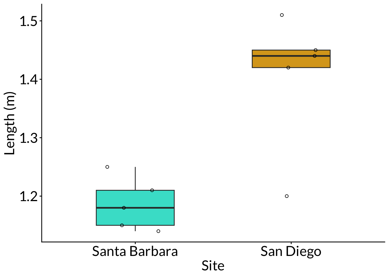
    Wilcoxon rank sum exact test

data:  length_m by site
W = 2, p-value = 0.03175
alternative hypothesis: true location shift is not equal to 0
Code
cliffs_delta( length_m ~ site,data = sharks)
r (rank biserial) |         95% CI
----------------------------------
-0.84             | [-0.96, -0.44]
b. Wilcoxon signed-rank
Code
# for a comparison of one group against a theoretical medianwilcox.test(Sample1, mu = theoretical)# for a comparison of two groupswilcox.test(value ~ sample,data = wilcox_df, paired =TRUE)
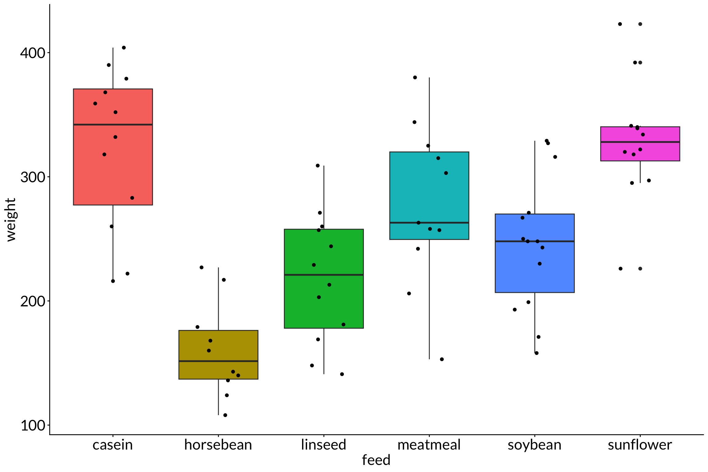
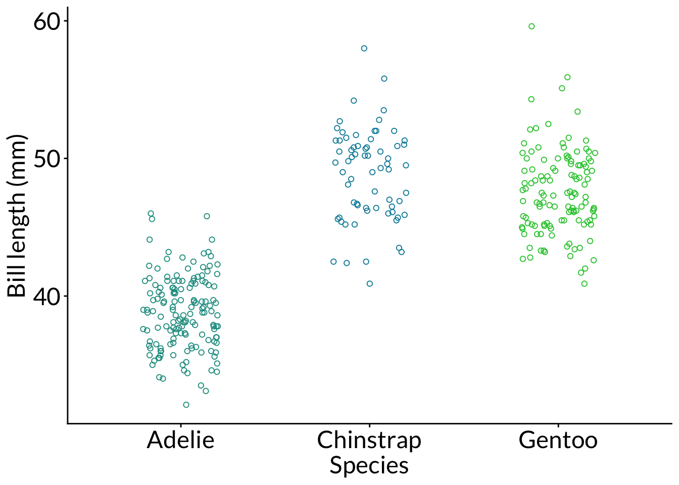
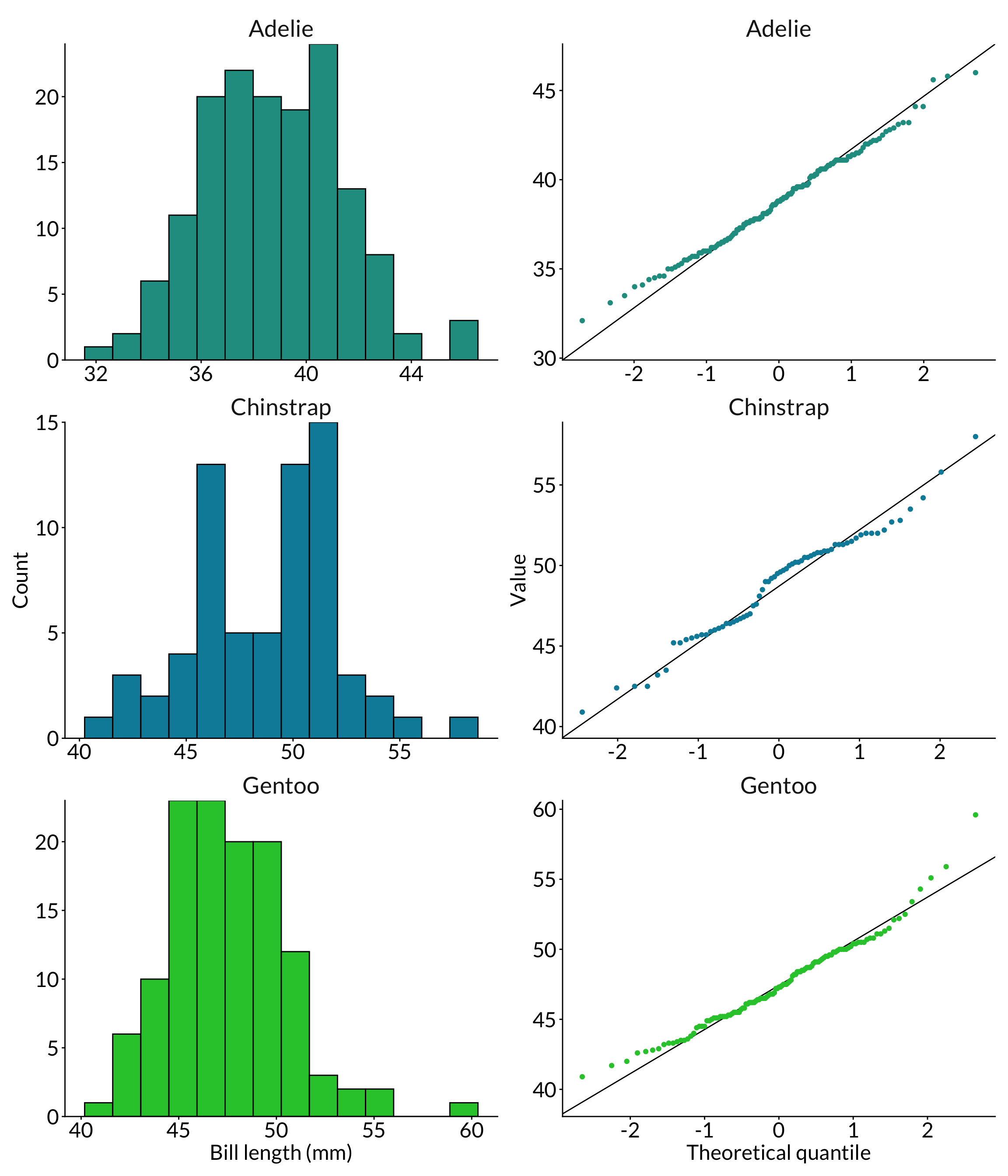
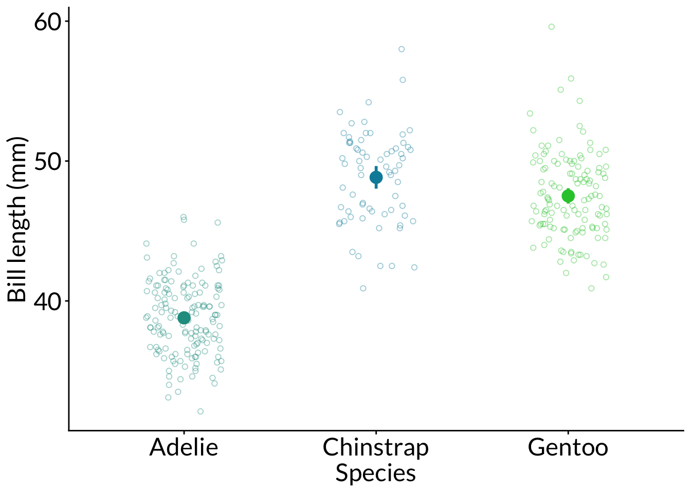
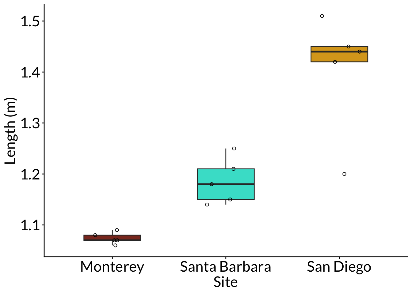
---title: "Week 5 figures - Lectures 9 and 10"date: 2026-02-03categories: [analysis of variance, eta squared, shapiro-wilk, levene, mann-whitney U, wilcoxon signed-rank, kruskal-wallis, cliffs delta]citation: url: https://winter-2026.envs-193ds.com/lecture/lecture_week-05.htmlengine: knitrknitr: opts_chunk: R.options: width: 120---## 0. Set up```{r set-up}#| message: false# cleaninglibrary(tidyverse)# visualizationtheme_set(theme_classic() + theme(panel.grid = element_blank(), axis.text = element_text(size = 18), axis.title = element_text(size = 18), text = element_text(family = "Lato")))library(patchwork)# datalibrary(palmerpenguins)# analysislibrary(car)library(effectsize)library(rstatix)library(dunn.test)```## 1. Math### a. sum of squaresAmong groups:$$\sum^k_{i = 1}\sum^n_{j = 1}(\bar{y_i} - \bar{y})^2$$where k is the number of groups, i is ith group, n is the number of observations per group, j is the jth observation. $\bar{y_i}$ is the mean of group i, while $\bar{y}$ is the grand mean (of all samples pooled together). Within groups:$$\sum^k_{i = 1}\sum^n_{j = 1}(y_{ij} - \bar{y_i})^2$$where $y_{ij}$ is the jth observation in the ith group, and $\bar{y_i}$ is the mean of group i. Total sum of squares: $$\sum^k_{i = 1}\sum^n_{j = 1}(y_{ij} - \bar{y})^2$$where $y_{ij}$ is the jth observation in the ith group, and $\bar{y}$ is the grand mean.### b. mean squaresAmong groups:$$\frac{SS_{among \ group}}{k - 1}$$Within groups: $$\frac{SS_{within \ group}}{n - k}$$### c. F-ratio/F-statistic$$\frac{MS_{among \ group}}{MS_{within \ group}}$$Put another way, the F-ratio is the ratio of among group variance to within group variance. If the among group variance is larger than within group variance, the F-ratio is large, and therefore the probability of among group variance being equal to within group variance is small. Thus, you would reject the null hypothesis if the F-ratio is large.### d. η squared$$\eta^2 = \frac{SS_{among \ group}}{SS_{among \ group} + SS_{within \ group}}$$### e. U statistic $$\begin{align}U_1 &= \Sigma R_1 - n_1(n_1 + 1)/2 = 17 - 5(5+1)/2 = 2 \\U_2 &= \Sigma R_2 - n_2(n_2 + 1)/2 = 38 - 5(5+1)/2 = 23\end{align}$$## 2. Warm up: code for a figure```{r chickwts-figure}#| fig-width: 12#| fig-height: 8# random sample of 10 rows from data framesample_n(chickwts, 10) %>% arrange(feed)ggplot(data = chickwts, # data frame: chickwts aes(x = feed, # x-axis: feed type y = weight, # y-axis: chick weight fill = feed)) + # fill by feed type geom_boxplot() + # creates a boxplot geom_jitter(height = 0, # prevents jitter from moving points along y-axis width = 0.2) + # narrows spread of jitter along x-axis theme(legend.position = "none") # removes legend```## 3. Analysis of varianceCentral question: How does bill length differ between penguin species?### a. Exploratory data visualization```{r penguins-explore}penguins_jitter <- ggplot(data = penguins, aes(x = species, y = bill_length_mm, color = species)) + geom_jitter(width = 0.2, height = 0, shape = 21) + scale_color_manual(values = c("#209c90", "#018ca9", "#27c839")) + labs(x = "Species", y = "Bill length (mm)") + theme(legend.position = "none")penguins_jitter```### b. histogram and qq plots```{r penguins-hist-and-qq}#| fig-width: 12#| fig-height: 14hist <- ggplot(data = penguins, aes(x = bill_length_mm, fill = species)) + geom_histogram(bins = 14, color = "black") + scale_fill_manual(values = c("#209c90", "#018ca9", "#27c839")) + scale_y_continuous(expand = c(0, 0)) + facet_wrap(~ species, scales = "free", ncol = 1) + labs(x = "Bill length (mm)", y = "Count") + theme(legend.position = "none", strip.background = element_rect(color = "white"), strip.text = element_text(size = 20))qq <- ggplot(data = penguins, aes(sample = bill_length_mm)) + geom_qq_line() + geom_qq(aes(color = species)) + scale_color_manual(values = c("#209c90", "#018ca9", "#27c839")) + facet_wrap(~ species, scales = "free", ncol = 1) + labs(x = "Theoretical quantile", y = "Value") + theme(legend.position = "none", strip.background = element_rect(color = "white"), strip.text = element_text(size = 20))hist + qq```### c. Shapiro-Wilk normality testGeneral: Is the response variable normally distributed? Example: Is bill length normally distributed?```{r penguins-shapiro-wilk}# first, wrangleadelie <- penguins %>% filter(species == "Adelie") %>% pull(bill_length_mm)chinstrap <- penguins %>% filter(species == "Chinstrap") %>% pull(bill_length_mm)gentoo <- penguins %>% filter(species == "Gentoo") %>% pull(bill_length_mm)# then, do the shapiro-wilk testshapiro.test(adelie)shapiro.test(chinstrap)shapiro.test(gentoo)```### d. Levene test of variancesGeneral: Are the group variances equal? Example: Are the species variances equal?```{r penguins-levene}leveneTest(bill_length_mm ~ species, data = penguins)``````{r penguins-var-calc}penguins |> drop_na(bill_length_mm) |> group_by(species) |> summarize(variance = var(bill_length_mm, na.rm = TRUE), n = length(bill_length_mm)) ```### e. analysis of variance```{r penguins-anova}# do the actual test# model object stored as `penguins_anova`penguins_anova <- aov(bill_length_mm ~ species, data = penguins)# output of the testpenguins_anova# more informationsummary(penguins_anova)```### f. post hoc testWhich group comparisons are different?```{r penguins-tukey-hsd}TukeyHSD(penguins_anova)```### g. effect size```{r penguins-eta-squared}eta_squared(penguins_anova)```### h. example of writingWithout the stats: Our results suggest a difference in bill length between species, with a large effect of species. Species differed in bill length, and pairwise comparisons between species showed that all three species differed from each other. Generally, Adelie penguins tend to have shorter bills than Chinstrap and Gentoo penguins. Gentoo penguins tend to have shorter bills than Chinstrap penguins.With the stats: Our results suggest a difference in bill length between species, with a large ($\eta^2$ = 0.71) effect of species. Species differed in bill length (one-way ANOVA, F(2, 339) = 410.6, p < 0.001, $\alpha$ = 0.05), and pairwise comparisons between species showed that all three species differed from each other. Generally, Adelie penguins tend to have 10.0 mm shorter bills than Chinstrap (Tukey HSD, p < 0.001, 95% confidence interval: [9.0, 11.1] mm) penguins and 8.7 mm shorter than Gentoo (Tukey HSD, p < 0.001, 95% confidence interval: [7.9, 9.6] mm) penguins. Gentoo penguins tend to have 1.3 mm shorter bills than Chinstrap penguins (Tukey HSD, p = 0.008, 95% confidence interval: [0.3, 2.4] mm). ### i. a "finalized" figure```{r penguins-final-fig}ggplot(data = penguins, aes(x = species, y = bill_length_mm, color = species)) + geom_jitter(width = 0.2, height = 0, shape = 21, alpha = 0.4) + stat_summary(geom = "pointrange", fun.data = mean_cl_normal, size = 0.8, linewidth = 1) + scale_color_manual(values = c("#209c90", "#018ca9", "#27c839")) + labs(x = "Species", y = "Bill length (mm)") + theme(legend.position = "none")```## 4. Non parametric tests### a. Mann-Whitney U```{r wilcox-example}sharks <- cbind(sb = c(1.25, 1.21, 1.18, 1.14, 1.15), sd = c(1.42, 1.44, 1.45, 1.51, 1.20)) %>% as_tibble() %>% pivot_longer(cols = sb:sd) %>% rename(site = name, length_m = value) |> mutate(site = case_match( site, "sb" ~ "Santa Barbara", "sd" ~ "San Diego" ), site = fct_relevel(as_factor(site), "Santa Barbara", "San Diego"))ggplot(data = sharks, aes(x = site, y = length_m)) + geom_boxplot(aes(fill = site), outliers = FALSE, width = 0.5) + geom_jitter( width = 0.2, height = 0, shape = 21 ) + labs(x = "Site", y = "Length (m)") + scale_fill_manual(values = c( "San Diego" = "goldenrod", "Santa Barbara" = "turquoise" )) + theme(legend.position = "none")wilcox.test( length_m ~ site, data = sharks)cliffs_delta( length_m ~ site, data = sharks)```### b. Wilcoxon signed-rank```{r wilcox-demo}#| eval: false# for a comparison of one group against a theoretical medianwilcox.test(Sample1, mu = theoretical)# for a comparison of two groupswilcox.test(value ~ sample, data = wilcox_df, paired = TRUE)```### c. Kruskal-Wallis```{r}sharks_monterey <-cbind(sb =c(1.25, 1.21, 1.18, 1.14, 1.15), sd =c(1.42, 1.44, 1.45, 1.51, 1.20),mt =c(1.09, 1.08, 1.07, 1.07, 1.06)) %>%as_tibble() %>%pivot_longer(cols = sb:mt) %>%rename(site = name,length_m = value) |>mutate(site =case_match( site,"sb"~"Santa Barbara","sd"~"San Diego","mt"~"Monterey" ),site =fct_relevel(as_factor(site), "Monterey", "Santa Barbara", "San Diego"))sharks_monterey |>group_by(site) |>summarize(median =median(length_m)) |>ungroup()kruskal.test( length_m ~ site,data = sharks_monterey)dunn_test( length_m ~ site,data = sharks_monterey,p.adjust.method ="bonferroni")dunn.test(x = sharks_monterey$length_m,g = sharks_monterey$site,method ="bonferroni")kruskal_effsize( length_m ~ site,data = sharks_monterey)ggplot(data = sharks_monterey,aes(x = site,y = length_m)) +geom_boxplot(aes(fill = site),outliers =FALSE,width =0.5) +geom_jitter(width =0.2,height =0,shape =21 ) +labs(x ="Site", y ="Length (m)") +scale_fill_manual(values =c("San Diego"="goldenrod","Santa Barbara"="turquoise","Monterey"="tomato4" )) +theme(legend.position ="none")``````{r}kruskal_df <-cbind(Sample1 =round(rnorm(n =5, mean =4, sd =1), 1), Sample2 =round(rnorm(n =5, mean =6, sd =1), 1),Sample3 =round(rnorm(n =5, mean =8, sd =1), 1)) %>%as_tibble() %>%pivot_longer(cols = Sample1:Sample3) %>%rename(sample = name) %>%arrange(sample)rank_by_hand <- kruskal_df %>%arrange(value) %>%rownames_to_column("ranks") %>%mutate(ranks =as.numeric(ranks)) %>%group_by(sample) %>%reframe(sum_ranks =sum(ranks))R1 <- rank_by_hand[1, 2]R2 <- rank_by_hand[2, 2]R3 <- rank_by_hand[3, 2]n <-15n1 <-5n2 <-5n3 <-5rstatix::kruskal_test(value ~ sample,data = kruskal_df)kruskal.test(value ~ sample,data = kruskal_df)#((12 * STATISTIC / (n * (n + 1)) - 3 * (n + 1)) / (1 - sum(TIES^3 - TIES) / (n^3 - n)))(12/(n*(n+1)))*((R1^2)/n1 + (R2^2)/n2 + (R3^2)/n3) -3*(n +1)rstatix::kruskal_effsize(value ~ sample,data = kruskal_df)rstatix::dunn_test(value ~ sample,data = kruskal_df)```