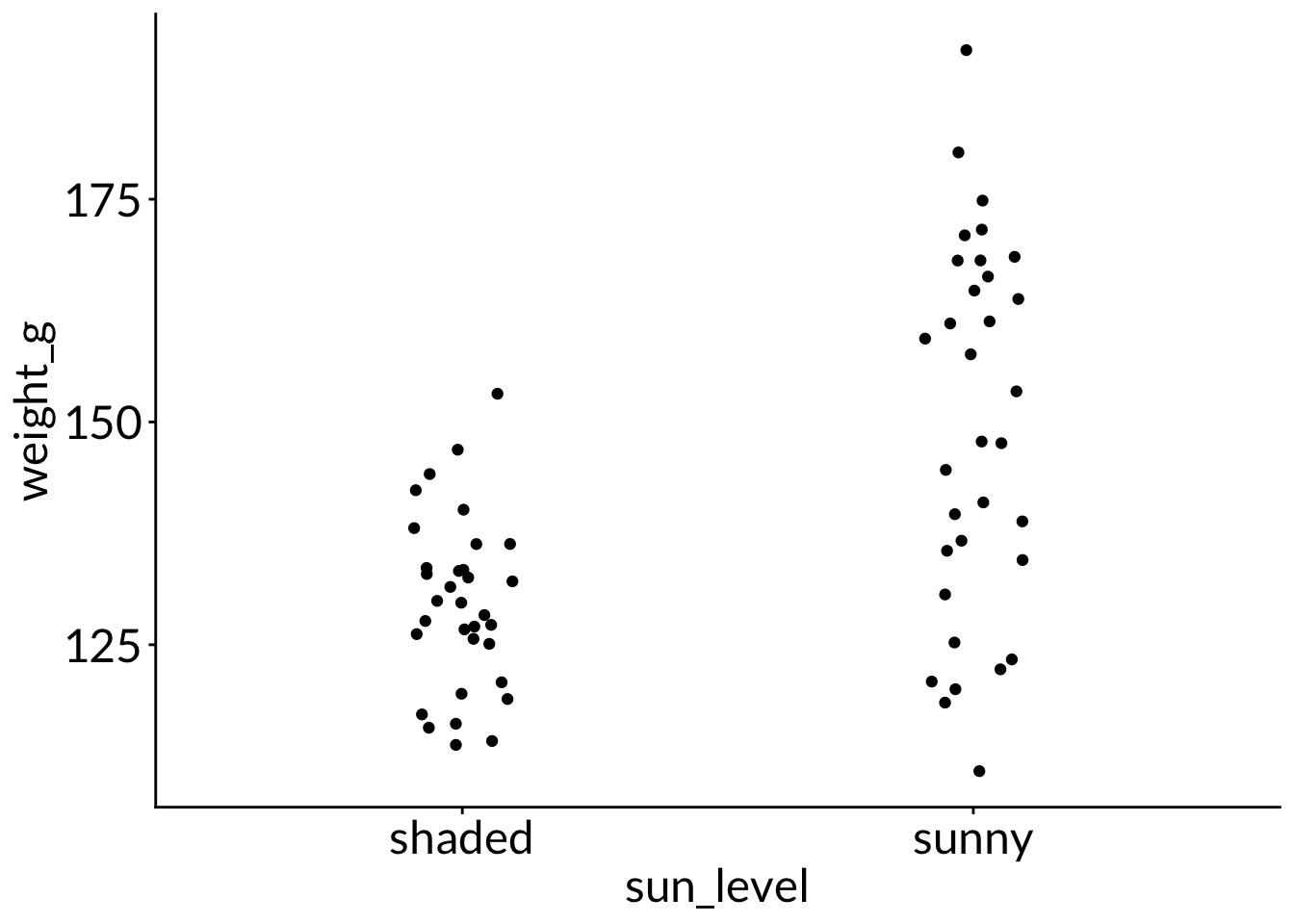
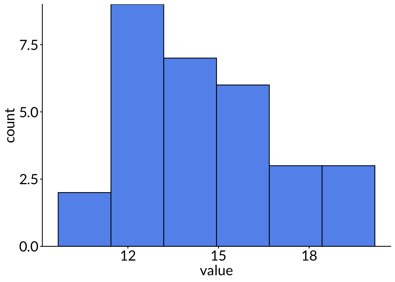
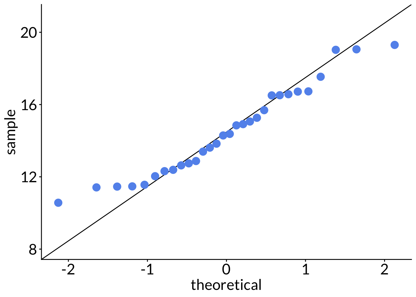
You have two raised beds in which you’re growing tomatoes. One bed is in the sun, but the other is in shade. You want to know if the weight of the tomatoes is different between beds. You measure 33 tomatoes from each bed.
    F test to compare two variances

data:  weight_g by sun_level
F = 0.21215, num df = 32, denom df = 32, p-value = 3.181e-05
alternative hypothesis: true ratio of variances is not equal to 1
95 percent confidence interval:
 0.1047793 0.4295538
sample estimates:
ratio of variances
         0.2121517
    Welch Two Sample t-test

data:  weight_g by sun_level
t = -4.8692, df = 44.993, p-value = 1.42e-05
alternative hypothesis: true difference in means between group shaded and group sunny is not equal to 0
95 percent confidence interval:
 -27.55166 -11.42803
sample estimates:
mean in group shaded  mean in group sunny
            129.5924             149.0822
3. Power analysis
Code
# higher powerpwr.t.test(n =NULL, d =0.7, sig.level =0.05, power =0.95)
     Two-sample t test power calculation

              n = 54.01938
              d = 0.7
      sig.level = 0.05
          power = 0.95
    alternative = two.sided

NOTE: n is number in *each* group
Code
# lower powerpwr.t.test(n =NULL, d =0.7, sig.level =0.05, power =0.80)
     Two-sample t test power calculation

              n = 33.02457
              d = 0.7
      sig.level = 0.05
          power = 0.8
    alternative = two.sided

NOTE: n is number in *each* group
4. Write about this result
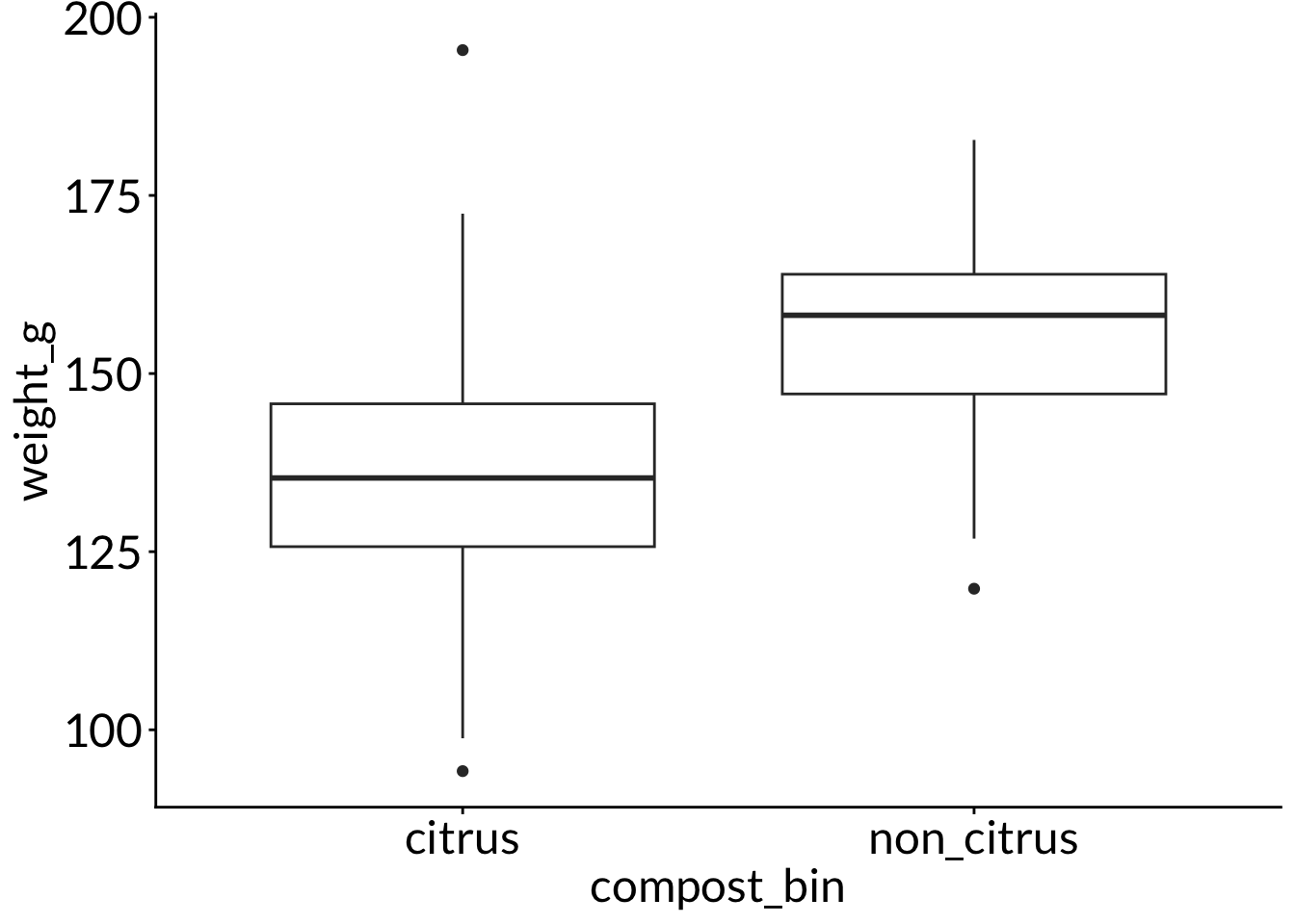
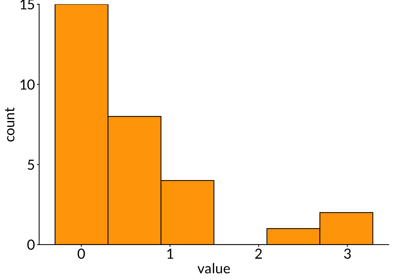
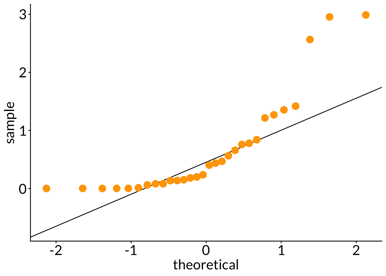
You have two worm compost bins: one in which you throw citrus peels, and the other in which you don’t. You’re curious to see if the citrus worms are bigger than the non-citrus worms. You measure 34 worms from each bin and find this result:
    F test to compare two variances

data:  weight_g by compost_bin
F = 2.2021, num df = 33, denom df = 33, p-value = 0.02627
alternative hypothesis: true ratio of variances is not equal to 1
95 percent confidence interval:
 1.099766 4.409198
sample estimates:
ratio of variances
          2.202064
    Welch Two Sample t-test

data:  weight_g by compost_bin
t = -4.8755, df = 57.848, p-value = 8.84e-06
alternative hypothesis: true difference in means between group citrus and group non_citrus is not equal to 0
95 percent confidence interval:
 -27.86552 -11.64356
sample estimates:
    mean in group citrus mean in group non_citrus
                136.0371                 155.7917
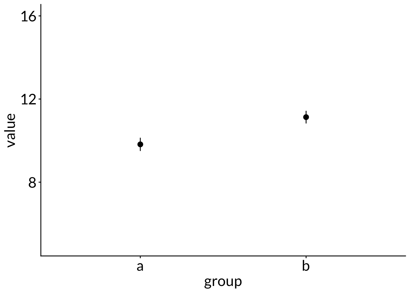
5. Effect size examples
a. large sample size, small difference
\[
\bar{y_a} - \bar{y_b}
\]
Code
set.seed(1)data <-cbind(a =rnorm(n =100, mean =10, sd =2), b =rnorm(n =100, mean =11, sd =2)) %>%as_tibble() %>%pivot_longer(cols =1:2, names_to ="group", values_to ="value") %>%group_by(group)set.seed(1)large <- data %>%slice_sample(n =40)ggplot(data = large,aes(x = group,y = value)) +stat_summary(geom ="pointrange",fun.data = mean_se) +scale_y_continuous(limits =c(5, 16))
    Two Sample t-test

data:  value by group
t = -2.9666, df = 78, p-value = 0.003996
alternative hypothesis: true difference in means between group a and group b is not equal to 0
95 percent confidence interval:
 -2.1892413 -0.4308888
sample estimates:
mean in group a mean in group b
       9.819199       11.129264
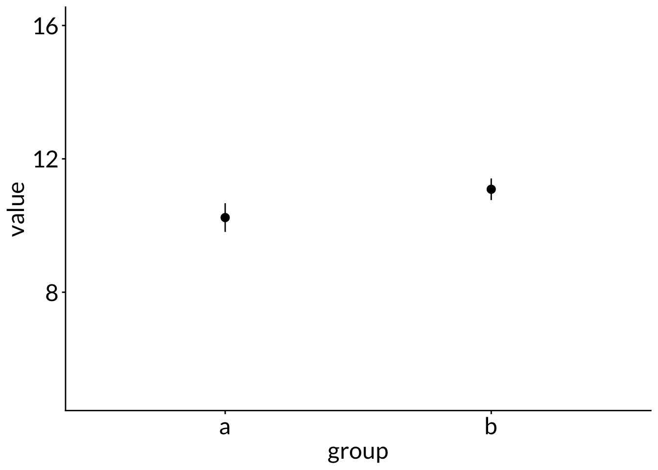
    Two Sample t-test

data:  value by group
t = -1.5737, df = 38, p-value = 0.1238
alternative hypothesis: true difference in means between group a and group b is not equal to 0
95 percent confidence interval:
 -1.9408171  0.2431029
sample estimates:
mean in group a mean in group b
       10.23925        11.08811
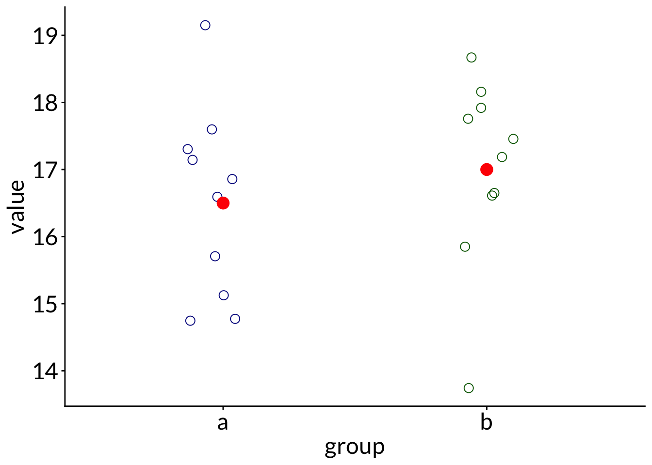
    Two Sample t-test

data:  value by group
t = -0.79057, df = 18, p-value = 0.4395
alternative hypothesis: true difference in means between group a and group b is not equal to 0
95 percent confidence interval:
 -1.8287398  0.8287398
sample estimates:
mean in group a mean in group b
           16.5            17.0
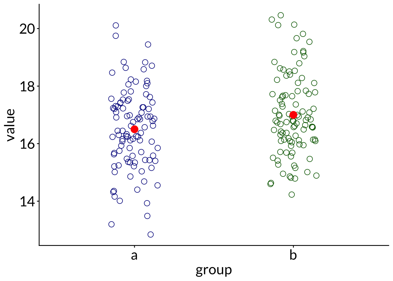
    Two Sample t-test

data:  value by group
t = -2.5, df = 198, p-value = 0.01323
alternative hypothesis: true difference in means between group a and group b is not equal to 0
95 percent confidence interval:
 -0.8944035 -0.1055965
sample estimates:
mean in group a mean in group b
           16.5            17.0
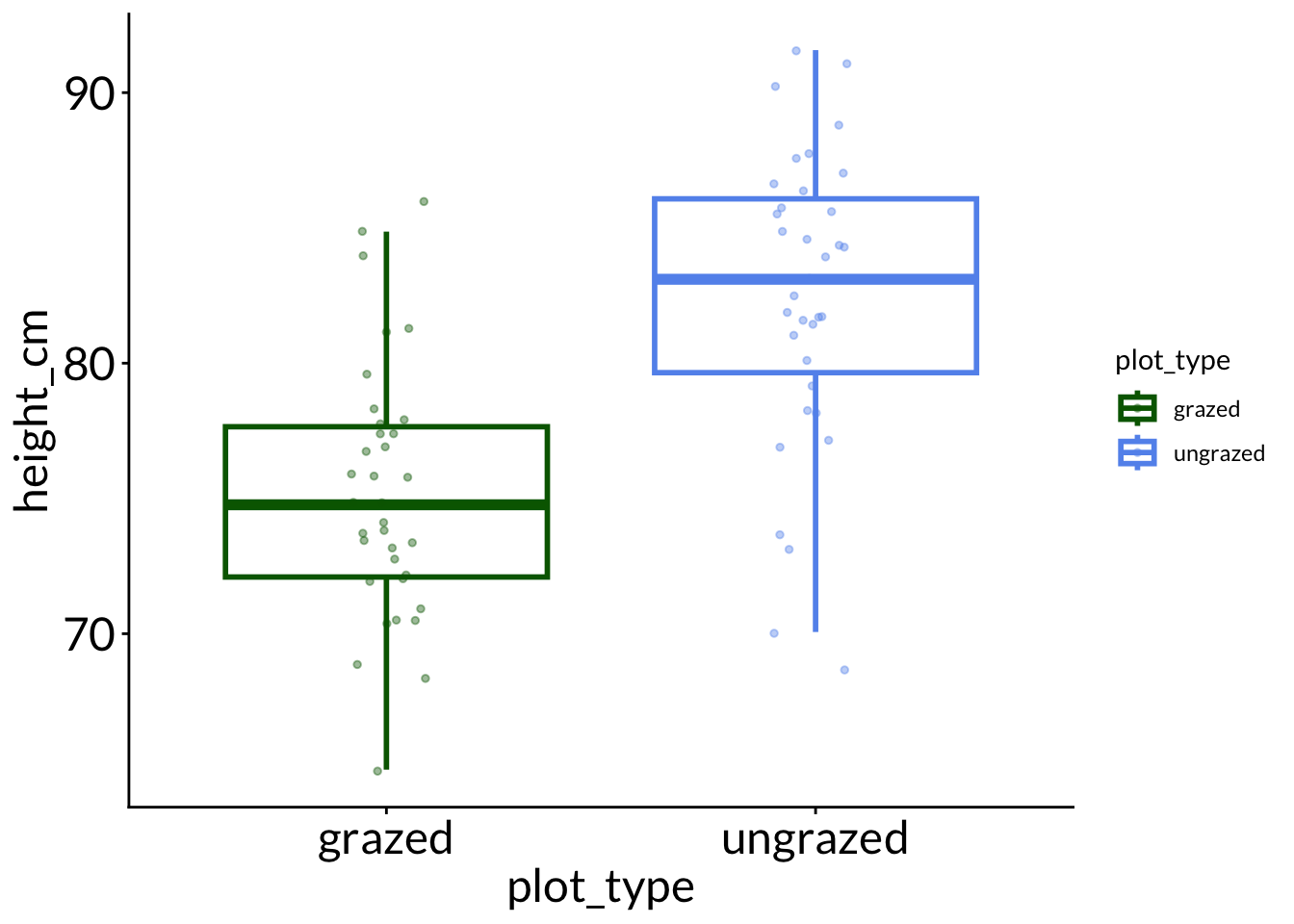
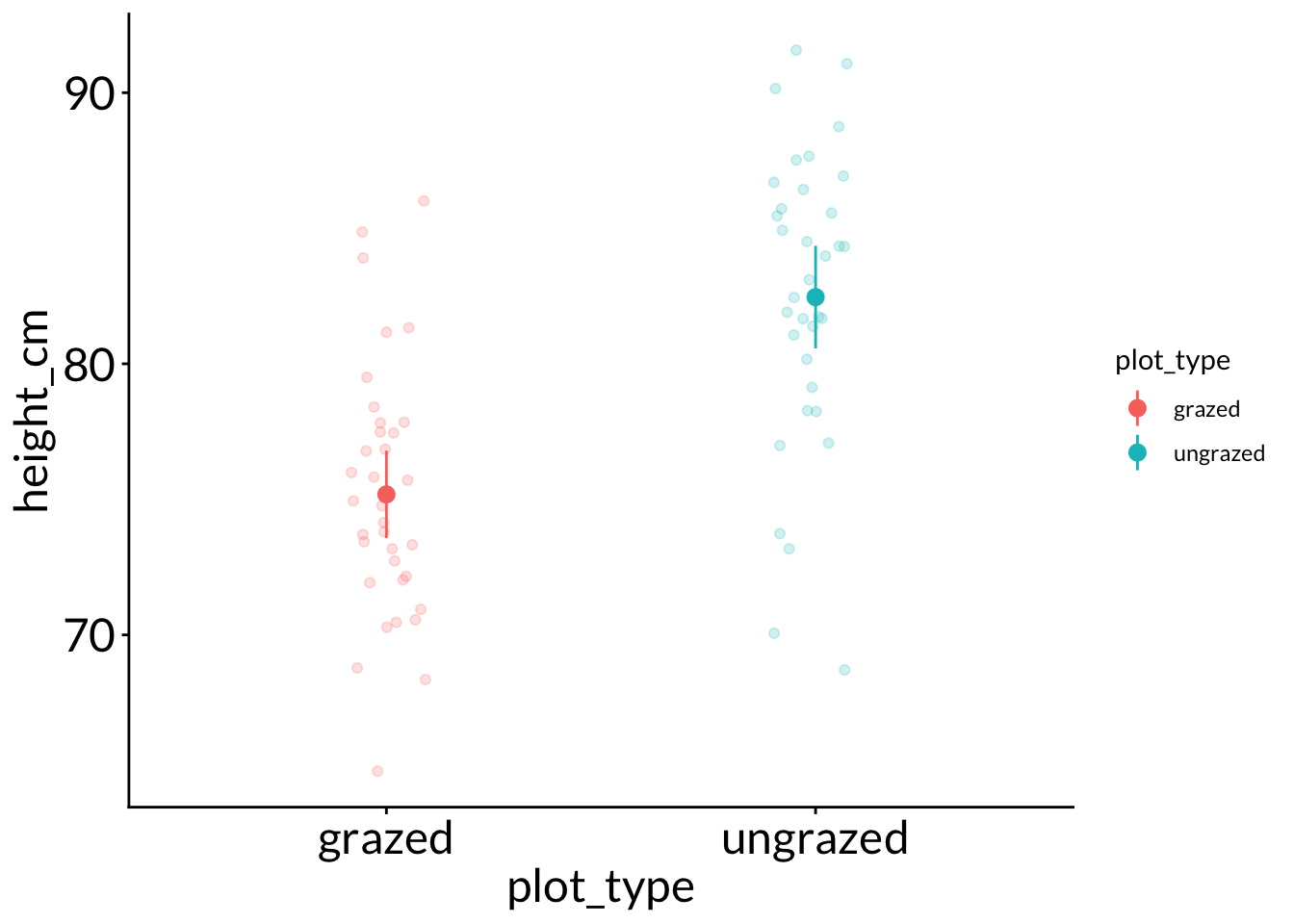
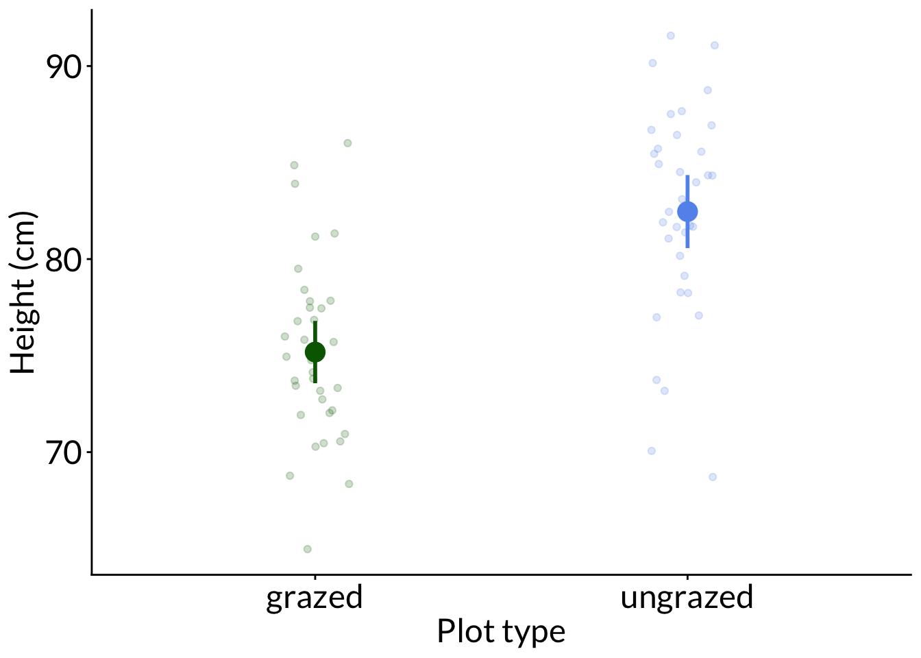
    F test to compare two variances

data:  height_cm by plot_type
F = 0.72641, num df = 34, denom df = 34, p-value = 0.3559
alternative hypothesis: true ratio of variances is not equal to 1
95 percent confidence interval:
 0.366669 1.439115
sample estimates:
ratio of variances
         0.7264149
    Two Sample t-test

data:  height_cm by plot_type
t = -5.9471, df = 68, p-value = 1.052e-07
alternative hypothesis: true difference in means between group grazed and group ungrazed is not equal to 0
95 percent confidence interval:
 -9.719086 -4.835512
sample estimates:
  mean in group grazed mean in group ungrazed
              75.18323               82.46053
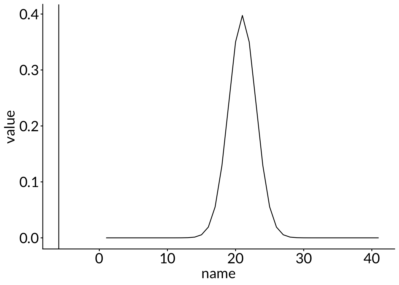
Code
vect <-dt(x =seq(from =-10, to =10, by =0.5), df =66.334) %>%enframe()ggplot(data = vect,aes(x = name,y = value)) +geom_line() +geom_vline(xintercept =-5.9471)
Cohen’s d:
Code
# pooled SDcohens_d( height_cm ~ plot_type,data = needlegrass,pooled_sd =TRUE)
Cohen's d |         95% CI
--------------------------
-1.42     | [-1.94, -0.89]

- Estimated using pooled SD.
    F test to compare two variances

data:  temp by treatment
F = 1.287, num df = 32, denom df = 29, p-value = 0.4953
alternative hypothesis: true ratio of variances is not equal to 1
95 percent confidence interval:
 0.6197933 2.6377877
sample estimates:
ratio of variances
          1.286962
Code
t.test(temp ~ treatment,data = pools)
    Welch Two Sample t-test

data:  temp by treatment
t = -11.206, df = 60.948, p-value < 2.2e-16
alternative hypothesis: true difference in means between group managed and group non-intervention is not equal to 0
95 percent confidence interval:
 -2.558536 -1.783706
sample estimates:
         mean in group managed mean in group non-intervention
                      4.952439                       7.123560
Code
cohens_d(temp ~ treatment,data = pools)
Cohen's d |         95% CI
--------------------------
-2.81     | [-3.51, -2.10]

- Estimated using pooled SD.
Statement: Our data suggest a difference in water temperature between managed (n = 33) and non-intervention (i.e. control, n = 30) vernal pools, with a strong (Cohen’s d = 2.19) effect of management.
Temperatures in managed pools were different from those in non-intervention pools (two-tailed two-sample t-test, t(60.9) = -8.7, p < 0.001, ⍺ = 0.05); on average, managed pools were 5.3 °C, while control pools were 7.1 °C.